After 30 years of teaching statistical methods in the geosciences, I would like to give a few tips for our next generation. Back then, I was in awe of a term like chi-square test and kept my hands off it for a long time. However, I could not avoid complicated methods such as spectral analysis and filtering, because my doctoral project was about signal processing of paleoceanographic time series. Here we go.
Step 1 – Data acquisition
One of the most common problems starts with the fact that the experiment used to generate the data does not match the questions – and ultimately also does not match the methods that are to be used to answer the questions (Trauth, 2021b). Do I have the necessary number of data points, the right (e.g. equidistant) sample scheme, is my time series long enough – these are questions that need to be answered long before static methods are used. Can I answer important questions about random and systematic errors with my data set? Do I need replicate measurements, possibly with a second measurement method? And what type of data does my measuring device generate, e.g. only 8-bit data, when I actually need much higher-resolution measured values, e.g. of the 64-bit double type?
Step 2 – Plot your data
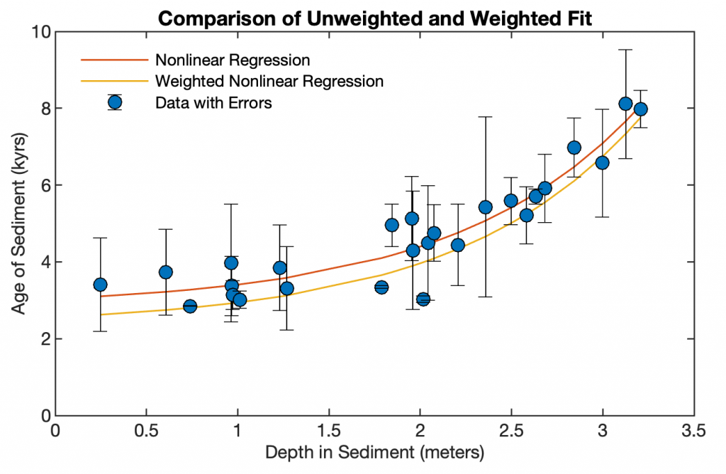
Once I have received my data from the measuring device, the first step is to examine it for inconsistencies and errors, possibly outliers. This can be done by looking through a table, but these are often very long and errors are overlooked. Simple plausibility tests help here, but above all simply a suitable graphical representation of the data (Trauth and Sillmann, 2018). Important trends should also become visible here, be it a linear or more complex trend, one or more cycles or events. We are often disappointed when expected trends, cycles or events are not found – and then hope that a sophisticated statistical method will be able to detect them. This often ends in disappointment and the trial and error of increasingly complicated methods.
Step 3 – Choose a method
The choice of method is often the result of advice from an advisor, colleagues or literature, such as textbooks or papers (Trauth, 2021b, 2022). This is where overly insistent advisors often show up, almost imposing their method (or the method they prefer to use). Don’t believe them, listen carefully and ask other colleagues before you come to an opinion yourself. There are fashions that emerge as quickly as they disappear, usually together with their proponents. The ongoing conflict between Bayesians and frequentists is a good example in statistics; warnings about the periodogram are another. If there were a perfect method, there would soon be no other, but even less suitable methods remain in the literature for a very long time. It is often colleagues who suggest a method that works well with their data, but this does not necessarily mean that it will work with your data.
Step 4 – Analyse your data
I recommend testing different methods with synthetic data that have similar properties to your data (Trauth, 2021b, 2022). Here you learn a lot about your data, the methods used, their strengths and weaknesses. If you do not get the expected result, e.g. an expected cycle, you may have made a mistake when selecting the sampling frequency. This is immediately apparent with synthetic data, but may not be the case with real data. When you use synthetic data with noise, you also learn a lot about how well the method can handle noise. How much noise can there be before you can no longer see your cycle? What influence do input parameters of the method (e.g. the length of the sliding window for evolutionary spectra) have on the expected result, especially those parameters for which there are no fixed recommendations? Once you have gained confidence in the data and the method, analyze the real data and compare the result with the synthetic data.
Step 5 – Documentation
Once you have completed your analyses, you must document them appropriately (Trauth and Sillmann, 2018). This includes a specification of the methods and all settings, as well as suitable graphical representations. Nowadays, scientific publications must be submitted not only with the original data – including outliers – but also with the computer code used. It is therefore important that this code is easy for readers to understand. You should use descriptive variable names, structure the scripts in a modular way and comment them well. The reader should be able to reproduce all analyses using the data and code, even after decades, and be able to select other parameters to estimate their influence on the result. Reproducibility is an important issue, all too often you read from doctoral students that their code no longer works after a few months and software updates.
Step 6 – Have a good cup of coffee
Now you are ready for a cup of good south Ethiopian coffee!

References
Trauth, M.H. (2021a) MATLAB Recipes for Earth Sciences – Fifth Edition. Springer International Publishing, 517 p., ISBN 978-3-030-38440-1. (MRES)
Trauth, M.H. (2021b) Signal and Noise in Geosciences, MATLAB Recipes for Data Acquisition in Earth Sciences. Springer International Publishing, 343 p., ISBN 978-3-030-74912-5 (MRDAES)
Trauth, M.H. (2022) Python Recipes for Earth Sciences – First Edition. Springer International Publishing, 403 p., Supplementary Electronic Material, Hardcover, ISBN 978-3-031-07718-0. (PRES)
Trauth, M.H., Sillmann, E. (2018) Collecting, Processing and Presenting Geoscientific Information, MATLAB® and Design Recipes for Earth Sciences – Second Edition. Springer International Publishing, 274 p., ISBN 978-3-662-56202-4. (MDRES)
