Create Publishable Graphics with MATLAB, Part 1 – MATLAB and Python Recipes for Earth Sciences

The graphics of MATLAB have been greatly improved since the very rustic plots of the early 1990s. In contrast to previous editions, in which all the graphics were edited by designer Elisabeth Sillmann (blaetterwaldDesign) with Adobe Illustrator, the majority of the graphics of the 4th edition of MRES were not processed after being exporting from MATLAB. Here is the script for creating a variant of Figure 4.9 from MRES.

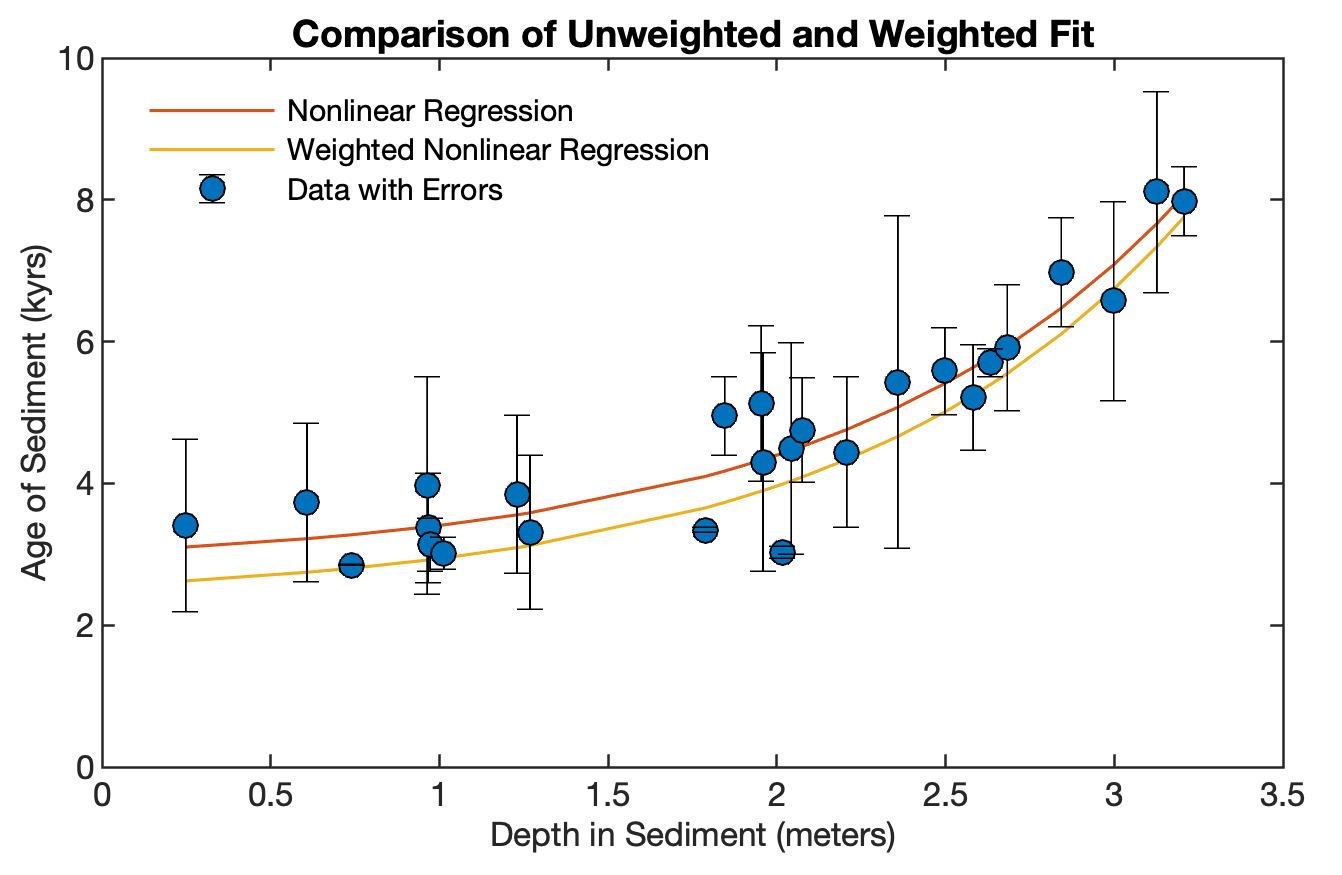
Figure 4.9 displays the result of nonlinear and weighted nonlinear regression by means of a synthetic example. Please read Chapter 4.10 of MRES if you wish to learn more about this type of analysis. We first generate a synthetic bivariate data set by typing

rng(0)
data(:,1) = 0.5 : 0.1 : 3;
data(:,1) = data(:,1) + 0.2*randn(size(data(:,1)));
data(:,2) = 3 + 0.2 * exp(data(:,1));
data(:,2) = data(:,2) + 0.5*randn(size(data(:,2)));
data = sortrows(data,1);

Next we run a nonlinear regression analysis to get the best fitted curve. We first generate synthetic error bars (in the 3rd column of data) and weights for the weighted regression (in the 4th column).

data(:,3) = abs(randn(size(data(:,1))));
data(:,4) = sum(data(:,3))./data(:,3);

The data can be also downloaded here. Now we run a unweighted and weighted nonlinear regression analysis to get another best fitted curve.

model = @(phi,t)(phi(1)*exp(t) + phi(2));
p0 = [0 0];
p = nlinfit(data(:,1),data(:,2),model,p0);
fittedcurve_1 = p(1)*exp(data(:,1)) + p(2);
model = @(phi,t)(phi(1)*exp(t) + phi(2));
p0 = [0 0];
p = nlinfit(data(:,1),data(:,2),...
   model,p0,'Weights',data(:,4))
fittedcurve_2 = p(1)*exp(data(:,1)) + p(2);

Now let us create a publishable graphics of the result. The MRES book does not explain how to create such sophisticated graphics, which is the topic of the MDRES book. Since the publication of the MDRES book, a new MATLAB graphics system was introduced in 2014, which is based on an improved infrastructure and although it supports most of the functionality of previous releases there are some differences.

Since then, graphics handles are now objects, not doubles. You can see an example in the script below, where the box around the legend is switched off by typing legend1.Box = ‘off’. Please read the excellent summary provided on the The MathWorks webpage about the new graphics system. That is why Elisabeth Sillmann and I am currently updating the MDRES book.

Advanced editing of graphics requires an understanding of the MATLAB requirement for graphics to be organized as hierarchical suites of graphics objects. Put simply, the hierarchies of graphical objects include four main layers: Root, Figure, Axes, and Chart and Primitive Objects.

The objects within each layer have a fixed set of properties, most of which can be modified to alter the appearance of a graph. In our example the graph consists of a root object, a figure object, an axes object, and a chart line object. The values of each set of properties can be queried and most of these values can be modified.

figure1 = figure(...
    'Position',[200 200 800 600],...
    'Color',[1 1 1]);
axes1 = axes(...
    'Box','on',...
    'XLim',[0 3.5],...
    'YLim',[0 10],...
    'Units','Centimeters',...
    'Position',[2 2 10 6],...
    'LineWidth',0.6,...
    'FontName','Helvetica',...
    'FontSize',8);
hold on
line1 = line(data(:,1),fittedcurve_1,...
    'LineWidth',0.75,...
    'Color',[0.8477 0.3242 0.0977]);
line2 = line(data(:,1),fittedcurve_2,...
    'LineWidth',0.75,...
    'Color',[0.9258 0.6914 0.1250]);
errorbar1 = errorbar(...
data(:,1),data(:,2),data(:,3),...
    'Marker','o',...
    'MarkerEdgeColor',[0 0 0],...
    'MarkerFaceColor',[0 0.4453 0.7383],...
    'Color',[0 0 0],...
    'LineStyle','none');
xlabel1 = xlabel(...
    'Depth in Sediment (meters)',...
    'FontName','Helvetica',...
    'FontSize',8);
ylabel1 = ylabel(...
    'Age of Sediment (kyrs)',...
    'FontName','Helvetica',...
    'FontSize',8);
title1 = title(...
    'Comparison of Unweighted and Weighted Fit',...
    'FontName','Helvetica',...
    'FontSize',9);
legend1 = legend('Nonlinear Regression',...
    'Weighted Nonlinear Regression',...
    'Data with Errors',...
    'Location','Northwest');
legend1.Box = 'off';

You can use the help for each of the commands to get the list of properties. For example, type help line in the Command Window, then click Reference page for line, then click Primitive Line Properties in the Help browser. You can export the graphics, for example, as Encapsulated Level 2 Color PostScript (EPSC2) file, as Portable Network Graphics (PNG) file with a resolution of 300 dpi.

print -depsc2 -cmyk afig_4_9.eps
print -dpng -r300 afig_4_9.png