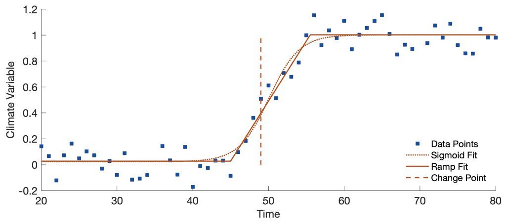
Detecting, measuring and classifying transitions in climate time series is one of the most important applications in modern time series analysis (Mudelsee, 2000; Trauth et al., 2018, 2021). Three methods are presented here: sigmoid fit, ramp fit and change point detection.
We can statistically analyze climate records for the amplitude, duration, and midpoint of a climate transition using three different methods. First, we fit a sigmoid function with m = 4 parameters a, b, c, and d
to the records xi with 1<i<n and n data points using nonlinear least-squares fitting. The sigmoid function (in its normalized representation) is a monotonic s-shaped curve, often referred to as a smooth version of a step function. The sigmoid function is bounded by two horizontal asymptotes xfit(t)→0 and 1 as t→–∞ and +∞, respectively. It has a bell-shaped first derivative curve and exactly one inflection point (parameter c), which can be interpreted as the midpoint of the transition.
Second, we statistically re-analyzed these records, fitting a ramp function again with m = 4 parameters x1, x2, t1, and t2.
to the n data points. The monotonic ramp-shaped curve has two horizontal pieces and an inclined piece, connected by two abrupt changes of direction and with a discontinuous first derivative.
Third, we can use findchangepts, which returns the largest number of changes in the mean, the standard deviation, and the trend of a time series (not exceeding a maximum number of permissible changes maxnumchg defined by the user) that minimize the sum of the residual error and an internal fixed penalty for each change. Here we use findchangepts to find a maximum number of maxnumchg=1 change points in the mean.
Before we used the three methods to fitting change-point models to the paleoenvironmental data, we teste them on a synthetic data set. This data set comprises 100 data points y for the period from t = 0 to t = 100, with a linear transition from y = 0 to y = 1 with a midpoint at t = 50. The linear transition within the synthetic time series starts at t = 46 and ends at t = 55, and has a slope of 1/10 and a y-intercept of –4.5. The y-values of the synthetic data sets are also superimposed by additive independent Gaussian noise with a mean of 0 and a standard deviation of 0.1. Such a data set can be generated with the following MATLAB script:
rng(0)
data(1:100,1) = 1 : 1 : 100;
data(1:45,2) = 0;
data(46:55,2) = 1/10 * data(46:55,1) - 4.5;
data(56:100,2) = 1;
data(:,2) = data(:,2) + 0.1*randn(size(data(:,2)));
The synthetic data set were then analyzed using the function fit together with fitoptions and fittype included in the Curve Fitting Toolbox of MATLAB to perform the nonlinear least-squares fitting (MathWorks, 2020) (Suppl. Fig. 1). We first fit a sigmoid function with four parameters a, b, c, and d, whose starting values we first define together with NonlinearLeastSquares using fitoptions:
fo = fitoptions('Method','NonlinearLeastSquares',...
    'StartPoint',[0 1 50 1]);
Next we define the model a+b*(1./(1+exp(-d*(x-c)))) in fittype
ft = fittype(@(a,b,c,d,x) ...
    a+b*(1./(1+exp(-d*(x-c)))),...
    'Coeff',{'a','b','c','d'},...
    'Options',fo);
before we use fit to find the best values for a, b, c, and d in a least-squares sense.
f1 = fit(data(:,1),data(:,2),ft)
The output of the fit function contains the best estimates of the four parameters a, b, c, and d, as well as several variables for estimating the quality of the result, including the RMSE, which we use within this study. Next, we use the same set of functions to fit a ramp function to the data. Since there is no ready-to-use ramp function available, we type
function x = rampfunction(t,t1,t2,x1,x2)
% RAMPFITMHT A line describing a ramp
% with two knickpoints at t1 and t2, where
% the value of variable changes from 1 to 0.

x = zeros(size(t));

for i = 1 : length(t)
    if t(i) < t1
        x(i) = x1;
    elseif t(i) >= t1 && t(i) < t2
        x(i) = x1 + (t(i)-t1)*(x2-x1)/(t2-t1);
    elseif t(i) >= t2
        x(i) = x2;
    end
end
end
and save it in the file with the name rampfunction.m. Using fitoptions, fittype and fit again
fo2 = fitoptions(...
    'Method','NonlinearLeastSquares',...
    'StartPoint',[45 55 0 1]);
ft2 = fittype('rampfunction(t,t1,t2,x1,x2)',...
    'Independent','t',...
    'Options',fo2);
f2 = fit(data(:,1),data(:,2),ft2)
we again get the best estimates of the four parameters t1, t2, x1 and x2. Alternatively, we can use the function RAMPFIT by Mudelsee (2000). Finally, we use findchangepts again to find the change point(s) in the data:
[ipoint,residual] = findchangepts(data(:,2),...
    'Statistic','mean',...
    'MinThreshold',0.8);
changepoints = data(ipoint,1);
close
m(1) = mean(data(1:ipoint(1),2));
for j = 1 : length(ipoint)-1
    m(j+1) = mean(data(ipoint(j):ipoint(j+1),2));
end
m(length(ipoint)+1) = mean(data(ipoint(j+1):end,2));
We can use the following code to display the data together with the results from our calculations:
% Figure Window and axes
figure('Position',[100 600 800 400])
axes('XLim',[20 80],...
    'YLim',[-.2 1.2],...
    'Position',[0.15 0.25 0.75 0.6],...
    'FontSize',14), hold on

% Sigmoid fit
p = plot(f1,data(:,1),data(:,2));
p(1).Color = [0.1 0.3 0.6];
p(1).Marker = 'Square';
p(1).MarkerSize = 6;
p(1).MarkerFaceColor = [0.1 0.3 0.6];
p(1).MarkerEdgeColor = [0.1 0.3 0.6];
p(2).Color = [0.7 0.3 0.1];
p(2).LineWidth = 1.5;
p(2).LineStyle = ':';

% Ramp fit
p = plot(f2,data(:,1),data(:,2));
p(1).Color = [0.1 0.3 0.6];
p(1).Marker = 'None';
p(2).Color = [0.7 0.3 0.1];
p(2).LineWidth = 1.5;
p(2).LineStyle = '-';

% Change Points
line([data(ipoint,1) data(ipoint,1)],[0 1],...
    'Color',[0.7 0.3 0.1],...
    'Marker','none',...
    'LineWidth',1.5,...
    'LineStyle','--')

% Labels
lgd = legend('Data Points','Sigmoid Fit',...
    '','Ramp Fit','Change Point');
lgd.Location = 'southeast';
lgd.Box = 'Off';
lgd.FontSize = 12;
lgd.AutoUpdate = 'Off';
xlabel('Time',...
    'FontSize',14)
ylabel('Climate Variable',...
    'FontSize',14)
References
Mudelsee, M., 2000. Ramp function regression: A tool for quantifying climate transitions. Computers and Geosciences 26, 1–15.
Trauth, M.H., Bergner, A.G.N., Foerster, V., Junginger, A., Maslin, M.A., Schaebitz, F., 2015. Episodes of Environmental Stability and Instability in Late Cenozoic Lake Records of Eastern Africa. Journal of Human Evolution, 87, 21-31.
Trauth, M.H., Foerster, V., Junginger, A., Asrat, A., Lamb, H., Schaebitz, F., 2018. Abrupt or Gradual? Change Point Analysis of the Late Pleistocene-Holocene Climate Record from Chew Bahir, Southern Ethiopia. Quaternary Research, 90, 321-330.
Trauth, M.H., Asrat, A., Berner, N., Bibi, F., Foerster, V., Grove, M., Kaboth-Bahr, S., Maslin, M., Mudelsee, M., Schaebitz, F., 2021. Northern Hemisphere Glaciation, African Climate and Human Evolution. Quaternary Science Reviews.
Trauth, M.H., 2021. MATLAB Recipes for Earth Sciences – Fifth Edition. Springer International Publishing, 517 p.
Trauth, M.H., 2022. Python Recipes for Earth Sciences – First Edition. Springer International Publishing, 403 p.


