
Paleoclimate time series are often very noisy due to the combined effect of low sedimentation rates, intensive bioturbation and small sample sizes (5-20 foraminifers). Adaptive filters may help to increase the signal-to-noise ratio of such time series where conventional methods such as fixed filters cannot be applied if optimal filtering is to be achieved, because the signal-to-noise ratio is unknown and varies with time.
On 5 March 2017 I posted an article on adaptive filtering using MATLAB. Since there is a section on adaptive filtering in the MRES book, there also is such a section in the new PRES book. Adaptive filters, which are widely used in the telecommunication industry. An adaptive filter is an inverse modeling process that iteratively adjusts its own coefficients automatically without requiring any a priori knowledge of the signal or the noise. Operating an adaptive filter involves (1) a filtering process whose purpose is to produce an output in response to a sequence of data and (2) an adaptive process that provides a mechanism for adaptively controlling the filter weights (Haykin 2003).
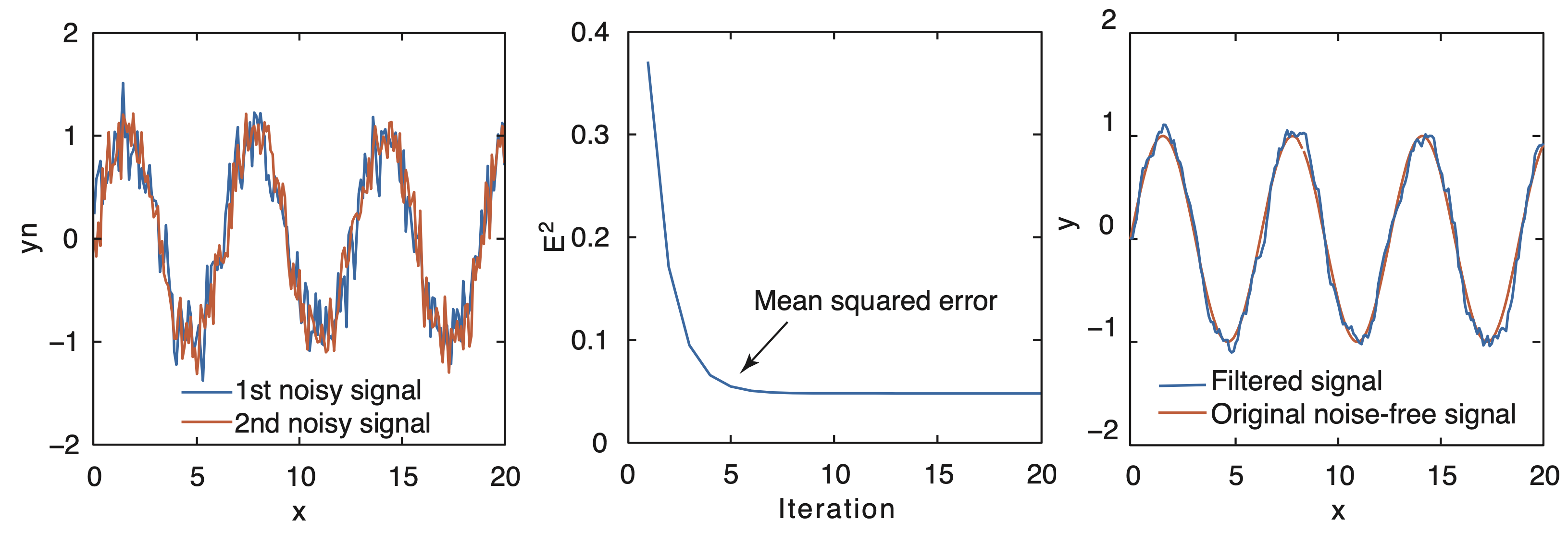
In the following example, which introduces canc(), each of these loop runs is called an iteration, and many loop runs are required if optimal results are to be achieved. This algorithm extracts the noise-free signal from two arrays x and s, which contain the correlated signals and uncorrelated noise. As an example, we generate two signals yn1 and yn2, which contain the same sine wave but different Gaussian noise:
import numpy as np
from numpy import linalg as lanalg
from canc import canc
from matplotlib import cm
import scipy.signal as signal
import matplotlib.pyplot as plt
from numpy.random import default_rng

x = np.linspace(0,100,1001)
y = np.sin(x)
rng = default_rng(0)
yn1 = y + 0.5*rng.standard_normal(y.shape)
yn2 = y + 0.5*rng.standard_normal(y.shape)

plt.figure()
plt.plot(x,yn1,x,yn2)
plt.show()
The algorithm canc() formats both signals, feeds them into the filter loop, corrects the signals for phase shifts, and formats the signals for the output. The required inputs are the signals x and s, the step size u, the filter length l, and the number of iterations iter. In our example, the two noisy signals are yn1 and yn2. We make an arbitrary choice of a filter with l=5 filter weights. A value of u in the range of 0 <u< l/emax (where emax is the largest eigenvalue of the autocorrelation matrix for the reference input) leads to reasonable results (Haykin 2003). The value of u is computed using
k = np.kron(yn1,np.transpose(yn1[None]))
w,v = lanalg.eig(k)
u = 1/np.max(w)
print(u)
where kron() returns the Kronecker tensor product of yn1 and yn1′ (which is a matrix formed by taking all possible products between the elements of yn1 and yn1′) and eig() returns the eigenvector of k. This yields
0.0013492697467229055
We now run the adaptive filter canc() for 20 iterations and use the value of u from above:
z,e,mer,w = canc(yn1,yn2,0.0013,5,20)
The output variables from canc() are the filtered primary signal z, the extracted noise e, the mean squared error mer for the number of iterations it performed with step size u, and the filter weights w for each data point in yn1 and yn2. The plot of the mean squared error mer
plt.figure()
plt.plot(mer)
plt.show()
illustrates the performance of the adaptive filter, although the chosen step size (u=0.0013) clearly results in a relatively rapid convergence. In most examples, a smaller step size decreases the rate of convergence but improves the quality of the final result. We therefore reduce u and run the filter again with further iterations:
z,e,mer,w = canc(yn1,yn2,0.0001,5,20)
The plot of the mean squared error mer against the iterations
plt.figure()
plt.plot(mer)
plt.show()
now converges after about six iterations. In practice, the user should vary the input arguments u and l in order to obtain the optimum result. We can now compare the filter output with the original noise-free signal:
plt.figure()
plt.plot(x,y,'b',x,z,'r')
plt.show()
This plot demonstrates that the noise level of the signal has been reduced dramatically by the filter. Next, the plot
plt.figure()
plt.plot(x,e,'r')
plt.show()
shows the noise extracted from the signal. Using the last output from canc(), we can calculate and display the mean filter weights of the final iteration from w:
wmean = np.mean(w,axis=0)

plt.figure()
plt.plot(wmean)
plt.show()
The frequency characteristic of the filter provides a more illustrative representation of the effect of the filter,
f,h = signal.freqz(wmean,1,worN=1024,fs=1)

plt.figure()
plt.plot(f,np.abs(h))
plt.show()
which shows that the filter is a lowpass filter with a relatively smooth transition band. This means that it does not have the quality of a recursive filter that was designed, for example, using the Butterworth approach. However, the filter weights are calculated in an optimization process rather than being chosen arbitrarily.
The strength of an adaptive filter lies in its ability to filter a time series with a variable signal-to-noise ratio along the time axis. Since the filter weight array W is updated for each individual data point, these filters are even used in real-time applications, such as in telecommunication systems. We examine this behavior through an example in which the signal-to-noise ratio in the middle of the time series (x=500) is reduced from about 10% to zero:
x = np.linspace(0,100,1001)
y = np.sin(x)
rng = default_rng(0)
yn1 = y + 0.5*rng.standard_normal(y.shape)
yn2 = y + 0.5*rng.standard_normal(y.shape)
yn1[501:] = y[501:]
yn2[501:] = y[501:]

plt.figure()
plt.plot(x,yn1,x,yn2)
plt.show()

k = np.kron(yn1,np.transpose(yn1[None]))
w,v = lanalg.eig(k)
u = 1 / np.max(w)
print(u)
which yields
0.0016086744408774288
We now run the adaptive filter canc() for 20 iterations and use the value of u from above:
z,e,mer,w = canc(yn1,yn2,0.0013,5,20)
The plot of the mean squared error mer versus the number of performed iterations it with step size u
plt.figure()
plt.plot(mer)
plt.show()
illustrates the performance of the adaptive filter, although the chosen step size u=0.0016 clearly results in a relatively rapid convergence. Again, we can now compare the filter output with the original noise-free signal:
plt.figure()
plt.plot(x,y,'b',x,z,'r')
plt.show()
This plot reveals that the filter output y is almost the same as the noise-free signal x. The plot
plt.figure()
plt.plot(x,e,'r')
plt.show()
shows the noise extracted from the signal. Here, we can observe some signal components that have been removed by the filter in error from within the noise-free segment of the time series beyond the change point in the signal-to-noise ratio.
References
Haykin S (2003) Adaptive Filter Theory. Prentice Hall, Englewood Cliffs, New Jersey.
Trauth, M.H. (1998) Noise removal from duplicate paleoceanographic time-series: The use of adaptive filtering techniques. Mathematical Geology, 30(5), 557-574. (MATLAB Code)
Trauth, M.H. (2021) MATLAB Recipes for Earth Sciences – Fifth Edition. Springer International Publishing, 517 p., ISBN 978-3-030-38440-1.
Trauth, M.H. (2022) Python Recipes for Earth Sciences – First Edition. Springer International Publishing, 403 p., Supplementary Electronic Material, Hardcover, ISBN 978-3-031-07718-0.
Widrow, B., Hoff, M., Jr. (1960) Adaptive switching circuits: IRE WESCON Conv. Rev., 4, 96-104.