
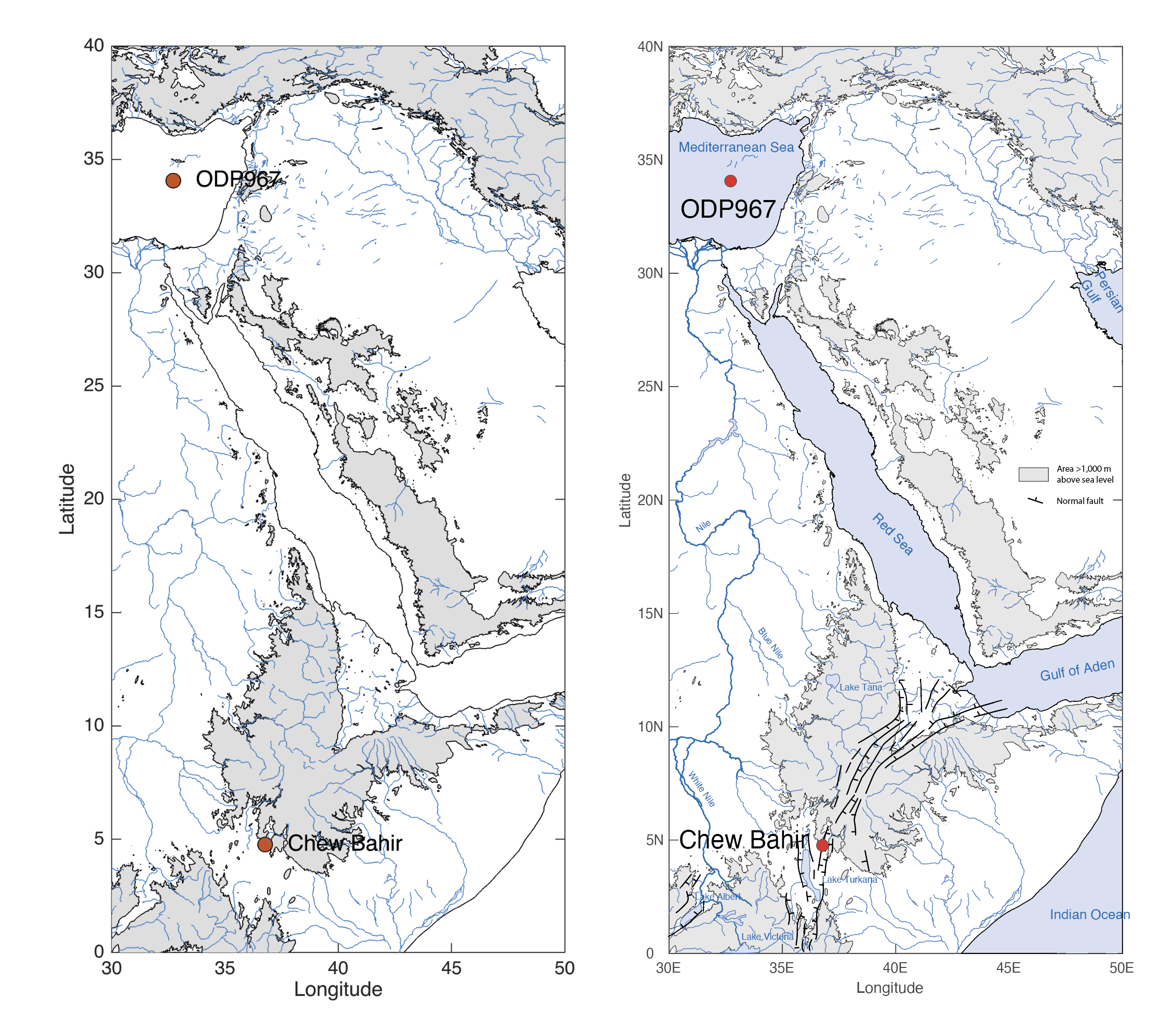
Variants of a map of northeastern Africa appear in recent publications (e.g., Trauth et al., 2021a, b) using coastlines from the GSHHG data set and topography from the ETOPO1 data set. Here I show how it was made.
In many earth science publications, there is a map showing drilling locations, sample points, or monitoring stations. There are countless ways to create such a map – typically a task for GIS software. As a MATLAB user, you would like to generate maps with the same software you used to perform your spatiotemporal analyses. Thanks to good graphics and toolboxes like the Mapping Toolbox from MathWorks, this is no problem. The geographic data needed for this is freely available, such as the GSHHG and ETOPO1 data sets used here.
The Global Self-consistent, Hierarchical, High-resolution Geography(GSHHG) database is an amalgamation of two public domain databases by Paul Wessel (SOEST, University of Hawaii, Honolulu, HI) and Walter Smith (NOAA Laboratory for Satellite Altimetry, Silver Spring, MD) (Wessel and Smith 1996). The format of the GSHHG changed and therefore the recipes contained in MRES and MDRES have to be modified.
The GSHHG database consists of the older GSHHS shoreline database (Soluri and Woodson 1990, Wessel and Smith 1996), which is a shoreline database, with the poor quality Antarctica data replaced by the more accurate data from Bohlander and Scambos (2007), and with rivers and borders taken from the CIA World Data Bank II (WDBII) (Gorny 1977). The GSHHG data can be downloaded from the SOEST server in three different formats: Generic Mapping Tools (GMT) files, ESRI shapefiles, or native binary files, and in a wide range of spatial resolutions. This example uses version 2.3.6 of the native binary file gshhg-bin-2.3.6.zip. We use the MATLAB unzip function to decompress this file
clear, clc, close all
unzip('gshhg-bin-2.3.6.zip')
which creates files containing the shorelines (gshhs), borders (wdb_borders) and rivers (wdb_rivers), each at different resolutions ranging from f (full resolution, 95.8 MB large) to c(crude resolution, 183 kb large), as explained on Paul Wessel’s SOEST webpage. As an example we import the high-resolution river data set from file wdb_rivers_h.b using
R = gshhs('gshhg-bin-2.3.7/wdb_rivers_h.b');
We obtain a structure array R which includes the longitude/latitude coordinates of the river segments together with various other types of information. We can extract, display and save the river coordinates by typing
clear river*
river(:,1) = R(1).Lon;
river(:,2) = R(1).Lat;
for i = 2 : 25776
clear river2
river2(:,1) = R(i).Lon;
river2(:,2) = R(i).Lat;
river = cat(1,river,river2);
end

plot(river(:,1),river(:,2))

save rivers.mat
For topography we use the 1 arc-minute global relief model of the Earth’s surface (ETOPO1) data set, which is discussed and visualized in Chapter 7.3 of my MRES book. The ETOPO1 data set is a global database of topographic and bathymetric data on a regular 1 arc-minute grid (about 2 km) (Amante and Eakins 2009). Older ETOPO2 and ETOPO5 global relief grids have been superseded but are still available. ETOPO1 is a compilation of data from a variety of sources. It can be downloaded from the NOAA National Centers for Environmental Information (NCEI) webpage. We can download either the whole-world grids, or custom grids for ice surface or bedrock. Here, we use the excerpt from the data set from the book, which can be downloaded here. We can import and flipud the data, as discussed in Chapter 7.3, and create a coordinate grid using
ETOPO1 = load('etopo1_data.txt');
ETOPO1 = flipud(ETOPO1);
[LON,LAT] = meshgrid(30:1/60:50,0:1/60:40);
The coastline and the rivers also come from the GSHHG database but we can also use the file coastline.mat from the book, which containes the coastlines of northeastern Africa. The rivers can also be downloaded from the file rivers.mat.
load coastline.mat
load rivers.mat
Then, we define the coordinates of the drill sites, Chew Bahir basin and ODP Site 967.
ODP967 = [32.7167 34.0667];
CHB = [36.7669 4.76125];
Finally, we create the map by typing
figure('Position',[100 100 600 800],...
   'Color',[1 1 1]);
axes('Box','on',...
   'DataAspectRatio',[1 1 1],...
   'XLim',[30 50],...
   'YLim',[0 40]);
line(data(:,1),data(:,2),...
   'Color',[0 0 0]);
xlabel('Longitude');
ylabel('Latitude');
hold on
contourf(LON,LAT,ETOPO1,[1000 1000])
line(ODP967(:,1),ODP967(:,2),...
   'Marker','o',...
   'MarkerSize',8,...
   'MarkerFaceColor',[0.8 0.3 0.1],...
   'MarkerEdgeColor',[0 0 0])
line(CHB(:,1),CHB(:,2),...
   'Marker','o',...
   'MarkerSize',8,...
   'MarkerFaceColor',[0.8 0.3 0.1],...
   'MarkerEdgeColor',[0 0 0])
line(river(:,1),river(:,2),...
   'Color',[0.1 0.5 0.8])
text(ODP967(:,1)+1,ODP967(:,2),'ODP967',...
   'FontSize',18)
text(CHB(:,1)+1,CHB(:,2),'Chew Bahir',...
   'FontSize',18)
colormap((gray).^0.2)
set(gca,'XLim',[30 50],...
   'YLim',[0 40]);

print -dpng -r600 chb_odp967_map_matlab.png
print -depsc2 chb_odp967_map_matlab.eps
We can view, edit and convert the graphic by using Adobe Illustrator or any other software to create the final design of the map (see file chb_odp967_map_illustrator.pdf for download).
References
Bohlander, J, Scambos T (2007) Antarctic coastlines and grounding line derived from MODIS Mosaic of Antarctica (MOA). National Snow and Ice Data Center, Boulder, Colorado
Soluri EA, Woodson VA (1990), World Vector Shoreline. International Hydrographic Review LXVII(1):27–35
Gorny AJ (1977) World Data Bank II General User Guide Rep. PB 271869. Central Intelligence Agency, Washington DC
Trauth, M.H., Asrat, A., Cohen, A., Duesing, W., Foerster, V., Kaboth-Bahr, S., Kraemer, H., Lamb, H., Marwan, N., Maslin, M., Schaebitz, F. (2021a) Recurring types of variability and transitions in the ~620 kyr record of climate change from the Chew Bahir basin, southern Ethiopia, Quaternary Science Reviews.
Trauth, M.H., Asrat, A., Berner, N., Bibi, F., Foerster, V., Grove, M., Kaboth-Bahr, S., Maslin, M., Mudelsee, M., Schaebitz, F. (2021b) Northern Hemisphere Glaciation, African Climate and Human Evolution. Quaternary Science Reviews.
Wessel P, Smith WHF (1996) A Global Self-consistent, Hierarchical, High-resolution Shoreline Database. Journal of Geophysical Research 101 B4: 8741-8743.