
Since 1 April 2016 all ASTER data products are free to all users. Here is an updated MATLAB script to import, enhance and georeference an ASTER image with MATLAB, different from that published in the 5th edition of MRES and the published earlier on this blog.
The ASTER sensor is mounted on the TERRA satellite launched in 1999, part of the Earth Observing System (EOS) series of multi-national NASA satellites (Abrams and Hook 2002). ASTER stands for Advanced Spaceborne Thermal Emission and Reflection Radiometer, providing high-resolution (15 to 90 meter) images of the Earth in 14 bands, including three visible to near-infrared bands (VNIR bands 1 to 3), six short-wave infrared bands (SWIR bands 4 to 9), and five thermal (or long-wave) infrared bands (TIR bands 10 to 14). ASTER images are used to map the surface temperature, emissivity, and reflectance of the Earth’s surface. The 3rd VNIR band is recorded twice: once with the sensor pointing directly downwards (band 3N, where N stands for nadir from the Arabic word for opposite), as it does for all other channels, and a second time with the sensor angled backwards at 27.6° (band 3B, where B stands for backward looking). These two bands are used to generate ASTER digital elevation models (DEMs).
The ASTER instrument produces two types of data: Level-1A (L1A) and Level-1B (L1B) data (Abrams and Hook 2002). Whereas the L1A data are reconstructed, unprocessed instrument data, the L1B data are radiometrically and geometrically corrected. Any data that ASTER has already acquired are available; they can be obtained from the webpage
https://earthexplorer.usgs.gov
As an example we process an image from an area in Kenya showing Lake Naivasha (0°46’31.38″S 36°22’17.31″E). The Level-1A data are stored in two files
AST_L1A_003_03082003080706_03242003202838.hdf
AST_L1A_003_03082003080706_03242003202838.hdf.met
The first file (116 MB) contains the actual raw data while the second file (102 kB) contains the header, together with all sorts of information about the data. We save both files in our working directory. Since the file name is very long, we first save it in the filename variable and then use filename instead of the long file name. We then need to modify only this single line of MATLAB code if we want to import and process other satellite images.
clear, close all, clc
filename = ...
  'AST_L1A_003_03082003080706_03242003202838.hdf';
The Image Processing Toolbox contains various tools for importing and processing files stored in the hierarchical data format (HDF). The graphical user interface (GUI) based import tool for importing certain parts of the raw data is
hdftool('filename')
This command opens a GUI that allows us to browse the content of the HDF-file, which obtains all information on the contents and imports certain frequency bands of the satellite image. Unfortunately, hdftool has been removed and causes an error message. The information that was previously provided by the function hdftool can now be obtained with the function hdfinfo
info = hdfinfo('filename')
which yields
info =

   struct with fields:
     Filename: 'naivasha.hdf'
   Attributes: [1×10 struct]
       Vgroup: [1×4 struct]
          SDS: [1×1 struct]
We can use
info.Vgroup
info.Vgroup.Name
info.Vgroup(2).Vgroup.Name
info.Vgroup(2).Vgroup(1).Vgroup.Name
info.Vgroup(2).Vgroup(1).Vgroup(2).SDS.Name
to dive into the hierarchical structure of the file to find out the names of the data fields that we want to import. We then use hdfread as a quicker way of accessing image data. The vnir_Band3n, vnir_Band2, and vnir_Band1 typically contain much information about lithology (including soils), vegetation, and surface water on the Earth’s surface. These bands are therefore usually combined into 24-bit rGB images. We first read the data
I1 = ...
  hdfread(filename,'VNIR_Band3N', ...
  'Fields','ImageData');
I2 = ...
  hdfread(filename,'VNIR_Band2', ...
  'Fields','ImageData');
I3 = ...
  hdfread(filename,'VNIR_Band1', ...
  'Fields','ImageData');
These commands generate three 8-bit image arrays, each representing the intensity within a certain infrared (IR) frequency band of a 4,200-by-4,100 pixel image. We are not using the data for quantitative analyses and therefore do not need to convert the digital number (DN) values into radiance and reflectance values. The ASTER User Handbook provides the necessary information on these conversions (Abrams and Hook 2002). Instead, we will process the ASTER image to create a georeferenced RGB composite of bands 3N, 2 and 1, to be used in fieldwork. We first use a contrast-limited adaptive histogram equalization method to enhance the contrast in the image by typing
I1 = adapthisteq(I1);
I2 = adapthisteq(I2);
I3 = adapthisteq(I3);
and then concatenate the result to a 24-bit rGB image using cat.
naivasha_rgb = cat(3,I1,I2,I3);
As with the previous examples, the 4,200-by-4,100-by-3 array can now be displayed using
imshow(naivasha_rgb,'InitialMagnification',10)
We set the initial magnification of this very large image to 10%. MATLAB scales images to fit the computer screen. Exporting the processed image from the Figure Window, we only save the image at the monitor’s resolution. To obtain an image at a higher resolution, we use the command
imwrite(naivasha_rgb,'naivasha.tif','tif')
This command saves the RGB composite as a TIFF-file naivasha.tif (ca. 52 MB) in the working directory, which can then be processed using other software such as Adobe Photoshop. The processed ASTER image does not yet have a coordinate system and therefore needs to be tied to a geographical reference frame (georeferencing). The header of the HDF file can be used to extract the geodetic coordinates of the four corners of the image contained in scenefourcorners.
UL = [-0.319922 36.214332];
LL = [-0.878267 36.096003];
UR = [-0.400443 36.770406];
LR = [-0.958743 36.652213];
From this we calculate the movingpoints with respect to the original image:
movingpoints(1,:) = ...
   [4100*(UL(2)-LL(2))/(UR(2)-LL(2)) 0];
movingpoints(2,:) = ...
   [0 4200*(UL(1)-LL(1))/(UL(1)-LR(1))];
movingpoints(3,:) = ...
   [4100 4200*(UL(1)-UR(1))/(UL(1)-LR(1))];
movingpoints(4,:) = ...
   [4100*(LR(2)-LL(2))/(UR(2)-LL(2)) 4200];
The four corners of the image correspond to the pixels in the four corners of the original image, which we store in a variable named fixedpoints.
fixedpoints(1,:) = [1 1];
fixedpoints(2,:) = [1 4200];
fixedpoints(3,:) = [4100 1];
fixedpoints(4,:) = [4100 4200];
The function fitgeotrans now takes the pairs of control points, movingpoints and fixedpoints, and uses them to infer a spatial transformation matrix tform. We use an affine transformation using affine which preserves points, straight lines and planes, and parallel lines remain parallel after transforming the image.
tform = fitgeotrans(fixedpoints, ...
   movingpoints,'affine');
Finally, the affine transformation can be applied to the original RGB composite naivasha_rgb in order to obtain a georeferenced version of the satellite image newnaivasha_rgb with the same size as naivasha_rgb using R from imref2d.
R = imref2d(size(naivasha_rgb));
newnaivasha_rgb=imwarp(naivasha_rgb,tform, ...
   'OutPutView',R);
An appropriate grid for the image can now be computed. The grid is typically defined by the minimum and maximum values for the longitude and latitude. The vector increments are then obtained by dividing the ranges of the longitude and latitude by the array’s dimensions reduced by one. Note the negative sign for southern latitudes.
X = 36.096003 : (36.770406 - ...
   36.096003)/4199 : 36.770406;
Y = -0.958743 : ( 0.958743 -  ...
   0.319922)/4099 : -0.319922;
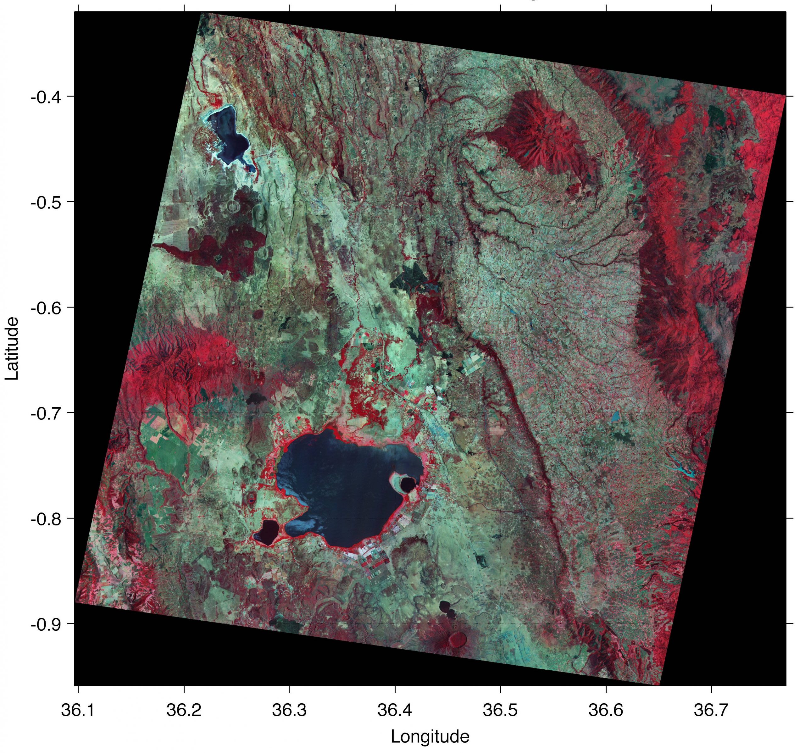
The georeferenced image is displayed with coordinates on the axes and a superimposed grid (Fig. 8.3). By default, the function imshow inverts the latitude axis when images are displayed by setting the YDir property to Reverse. To invert the latitude axis direction back to normal, we need to set the YDir property to Normal by typing
imshow(flipud(newnaivasha_rgb),...
    'XData',X,...
    'YData',Y,...
    'InitialMagnification',30)
axis on, grid on, set(gca,'YDir','Normal')
xlabel('Longitude'), ylabel('Latitude')
title('Georeferenced ASTER Image')
Exporting the image is possible in many different ways, for example using
print -djpeg70 -r600 naivasha_georef.jpg
to export it as a JPEG file naivasha_georef.jpg, compressed to 70% and with a resolution of 600 dpi.
References
Trauth, M.H. (2021) MATLAB Recipes for Earth Sciences – Fifth Edition. Springer International Publishing, ~500 p., Supplementary Electronic Material, Hardcover, ISBN: 978-3-030-38440-1.