
 Since 1 April 2016 all ASTER data products are free to all users. Here is an example, different from the one described in the MRES book, to demonstrate how to import, enhance and georeference an ASTER image with MATLAB.
The Advanced Spaceborne Thermal Emission and Reflection Radiometer (ASTER) sensor is mounted on the TERRA satellite launched in 1999, part of the Earth Observing System (EOS) series of multi-national NASA satellites (Abrams and Hook 2002). ASTER provides high-resolution (15 to 90 meter) images of the earth in 14 bands, including three visible to near infrared bands (VNIR bands 1 to 3), six short-wave infrared bands (SWIR bands 4 to 9), and five thermal (or long-wave) infrared bands (TIR bands 10 to 14).
ASTER images are used to map the surface temperature, emissivity, and reflectance of the earth’s surface. The 3rd near infrared band is recorded twice: once with the sensor pointing directly downwards (band 3N, where N stands for nadir from the Arabic word for opposite), as it does for all other channels, and a second time with the sensor angled backwards at 27.6° (band 3B, where B stands for backward looking). These two bands are used to generate ASTER digital elevation models (DEMs).
As an example we process an image from an area in Kenya showing Lake Baringo. These images, as well as all other ASTER products, are now available through from variable sources listed on the ASTER webpage. I use the NASA Reverb and the Earth Explorer to search and download ASTER data and other digital data of the Earth.
As an example we use an image of Lake Baringo stored in the file with a very long name. The example comes from a larger MATLAB script with which multiple ASTER images are processed at the same time wherein the example described here is image #24.
clear, clc
filename24 = ...
    'AST_L1B_003_02012002080830_02192002105819.hdf';
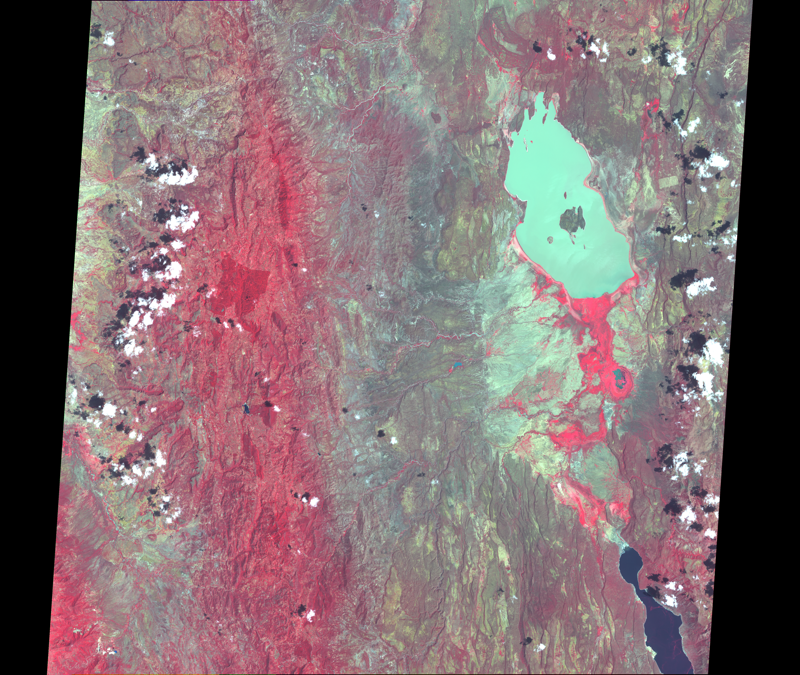
The Image Processing Toolbox contains various tools for importing and processing files stored in the hierarchical data format (HDF). The vnir_Band3n, vnir_Band2, and vnir_Band1 typically contain much information about lithology (including soils), vegetation and water on the earth’s surface. These bands are therefore usually combined into 24-bit RGB images. We first read the data
I1_24 = hdfread(filename24,...
    'VNIR_Swath','Fields','ImageData3N');
I2_24 = hdfread(filename24,...
    'VNIR_Swath','Fields','ImageData2');
I3_24 = hdfread(filename24,...
    'VNIR_Swath','Fields','ImageData1');
adjust image intensity values
I1_24 = imadjust(I1_24);
I2_24 = imadjust(I2_24);
I3_24 = imadjust(I3_24);
and then concatenate the result to a 24-bit RGB image using cat.
Image_24 = cat(3,I1_24,I2_24,I3_24);
Then we display the RGB composite of the ASTER image and save it to the harddrive:
figure('Position',[50 350 600 600],...
    'Color',[1 1 1])
Image_24 = imadjust(Image_24,stretchlim(Image_24));
imshow(Image_24,'InitialMagnification',20)
imwrite(Image_24,'image_24.tif','tif')
The processed ASTER image does not yet have a coordinate system and therefore needs to be tied to a geographical reference frame (georeferencing). The HDF browser
hdftool(filename)
can be used to extract the geodetic coordinates of the four corners of the image. This information is contained in the header of the HDF file. Having launched the HDF tool, we select on the uppermost directory and find a long list of file attributes in the upper right panel of the GUI, one of which is productmetadata.0, which includes the attribute scenefourcorners. We collect the coordinates of the four scene corners into a single array inputpoints.
inputpoints(1,:) = [35.6254 0.8690];
inputpoints(2,:) = [35.5447 0.3054];
inputpoints(3,:) = [36.289 0.7725];
inputpoints(4,:) = [36.2084 0.2093];
The four corners of the image correspond to the pixels in the four corners of the image, which we store in a variable named basepoints.
basepoints(1,:) = [1,4980];
basepoints(2,:) = [1,1];
basepoints(3,:) = [4200,4980];
basepoints(4,:) = [4200,1];
Using an affine transformation we can actually georeference the ASTER image of the Baringo basin.
tform = fitgeotrans(inputpoints,basepoints,...
    'affine');
xLimitsIn = 0.5 + [0 size(Image_24,2)];
yLimitsIn = 0.5 + [0 size(Image_24,1)];
[XBounds,YBounds] = ...
     outputLimits(tform,xLimitsIn,yLimitsIn);
Rout = imref2d(size(Image_24),XBounds,YBounds);
newImage_24 = imwarp(Image_24,tform,...
     'OutputView',Rout);
X = 35.5447 : (36.289-35.5447)/4980 : 36.289;
Y = 0.2093 : (0.8690-0.2093)/4200 : 0.8690;
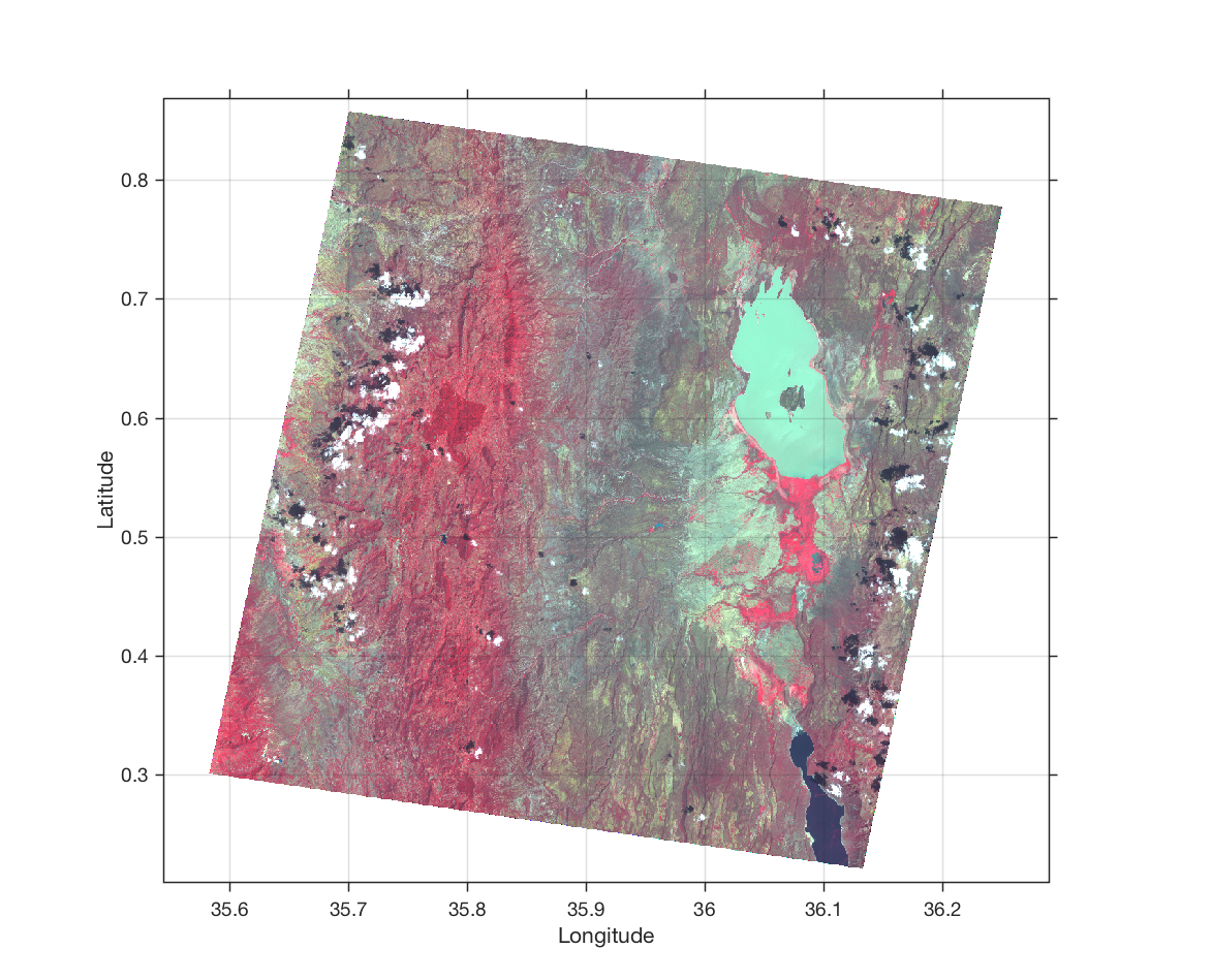
Please read Chapter 8.5 of the MRES book if you wish to learn more about this transformation. We can display and export the image using
figure('Position',[50 350 600 600],...
    'Color',[1 1 1])
imshow(flipud(newImage_24),...
    'XData',X,...
    'YData',Y,...
    'InitialMagnification',20)
set(gca,'YDir','Normal',...
    'FontSize',14,...
    'Visible','On',...
    'XGrid','On',...
    'YGrid','On',...
    'LineWidth',1.5,...
    'FontSize',18,...
    'Position',[0.1 0.1 0.8 0.8])
xlabel('Longitude'), ylabel('Latitude')
print -dpng -r75 image_24_georef_1.png
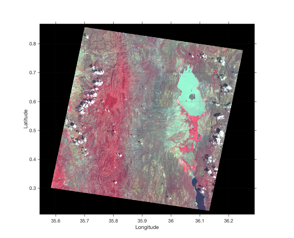 This image has a large black areas which are not very printer friendly. If you wish to print it on a larger plotter and take it to the field your departmental drawing office will appreciate a version of the image with all black replaced by white. Be careful if your image has lots of black pixels. You can also the magic pen of an image processing software to remove the black areas before printing.
newImage_24(newImage_24==0) = 255;
Here is the version with white areas around the actual image:
figure('Position',[50 350 600 600],...
    'Color',[1 1 1])
imshow(flipud(newImage_24),...
    'XData',X,...
    'YData',Y,...
    'InitialMagnification',20)
set(gca,'YDir','Normal',...
    'FontSize',14,...
    'Visible','On',...
    'XGrid','On',...
    'YGrid','On',...
    'LineWidth',1.5,...
    'FontSize',18,...
    'Position',[0.1 0.1 0.8 0.8])
xlabel('Longitude'), ylabel('Latitude')
print -dpng -r75 image_24_georef_2.png
References
Abrams M, Hook S (2002) ASTER User Handbook – Version 2. Jet Propulsion Laboratory and EROS Data Center, Sioux Falls