When I was working on the student experiments for the book Signal and Noise in Geosciences (Springer 2021), there was an inexpensive 3D scanner available – right up until that moment when I got the money to actually buy it. The company Hewlett Packard bought the smaller manufacturing company and stopped the production of the cheap scanner. HP was selling much more expensive 3D scanners at that time. Now there is a inexpensive 3D scanner again, the Revopoint MINI, and I just got one. Here are the first results, scanning with the company’s software, then importing, processing and displaying the point cloud with texture with MATLAB.
I got the Revopoint MINI with the Portable Turntable, downloaded the free RevoScan software and plugged everything together. The rather simple turntable rotates at a constant speed, which you can change once you’ve connected it. The manuals for the Revopoint MINI are quite good, available for download at the company’s webpage. There are also a number of great YouTube Videos with step-by-step instructions. I tried to scan the first object, of course without reading the instructions, and quickly realized that reading the manual is always a good advise.
As soon as you launched the software for the first time, you are asked to update the firmware of the camera. After updating the firmware, the camera sends out blue light, captures a 3D preview from the Depth Camera and a photo from the RGB Camera. The scanner can output models with a 0.05 mm point distance and a single-frame precision of up to 0.02 mm. Together with the RGB image, which colors the points of the dots, you get a colored 3D model of the object, in our example a light-colored seashell.
The graphical user interface of the software has several push buttons, including the one to start the scanning process. After pressingn the Scan button, we can set the Accuracy to High Accuracy Scan, the Scan Mode to Features, the Texture to Color, and the Accessories to None in the pop-up window entitled New Project. After pressing OK, we switch to a different interface, with previews of the two camera systems on the left, the rotating object to be scanned in the middle, and several push buttons on the right.
In order to get good results, too much ambient light should be avoided. We can leave the brightness of the RGB Camera at Auto. The Depth Camera, however, needs to be carefully adjusted to get good results, by moving the slider so that neither blue nor red pixels are visible (or as few of them as possible). The object to be scanned should be within the rectangular grid of red lines in the RGB Camera preview.
We then push the Start button, indicated with a blue triangle on the right, to start the scanning process. When the object has completed one full round we can press the Stop button, indicated with a blue square. In the pop-up window we disable the Fuse the point cloud immediately option and press Complete. Below the Start and Stop button we press the small black triangle of the Fuse button to change the Point pitch (mm) to the smallest possible value of 0.02 mm. We then press the X in the pop-up window and press the Fuse button right of the triangle.
We then press the small black triangle of the Mesh button and change the Settings to Manual, change Mesh Quality fo Maximum of 6.0, Denoise to 3 and enable the FIll Holes option. We then press the X in the pop-up window and press the Mesh button right of the triangle. The software stores all files in a directory named in the model-y-m-d-h-m-s format. We can use the Export button to save the 3D model with texture in the PLY and OBJ format, 3D models without texture also in the STL format. We export our 3D model to a file named seashell_fuse.ply.
We can then use the free RevoStudio Software to preview and edit the 3D scan. The software requires a verification key, which is sent as soon as you enter an email address above and send it. The software runs smoothly and provides a number of useful features. There are many other software tools such as CloudCompare to display and process point clouds. Alternatively, MATLAB offers a wide range of algorithms for processing point clouds, e.g. Structure for Motion algorithms, which are included in the Computer Vision Toolbox and the Lidar Toolbox, among others.
For example, the pcread function can be used to read in point clouds.
pcshellfuse = pcread('seashell_fuse.ply')
The function creates a pointCloud object that we call pcshellfuse. We can access its proporties if we do not terminate the statement with a semicolon:
pointCloud with properties:

Location: [190436×3 single]
Count: 190436
XLimits: [14.8615 77.3469]
YLimits: [-21.9052 21.2096]
ZLimits: [-197.8961 -145.0877]
Color: [190436×3 uint8]
Normal: [190436×3 single]
Intensity: []
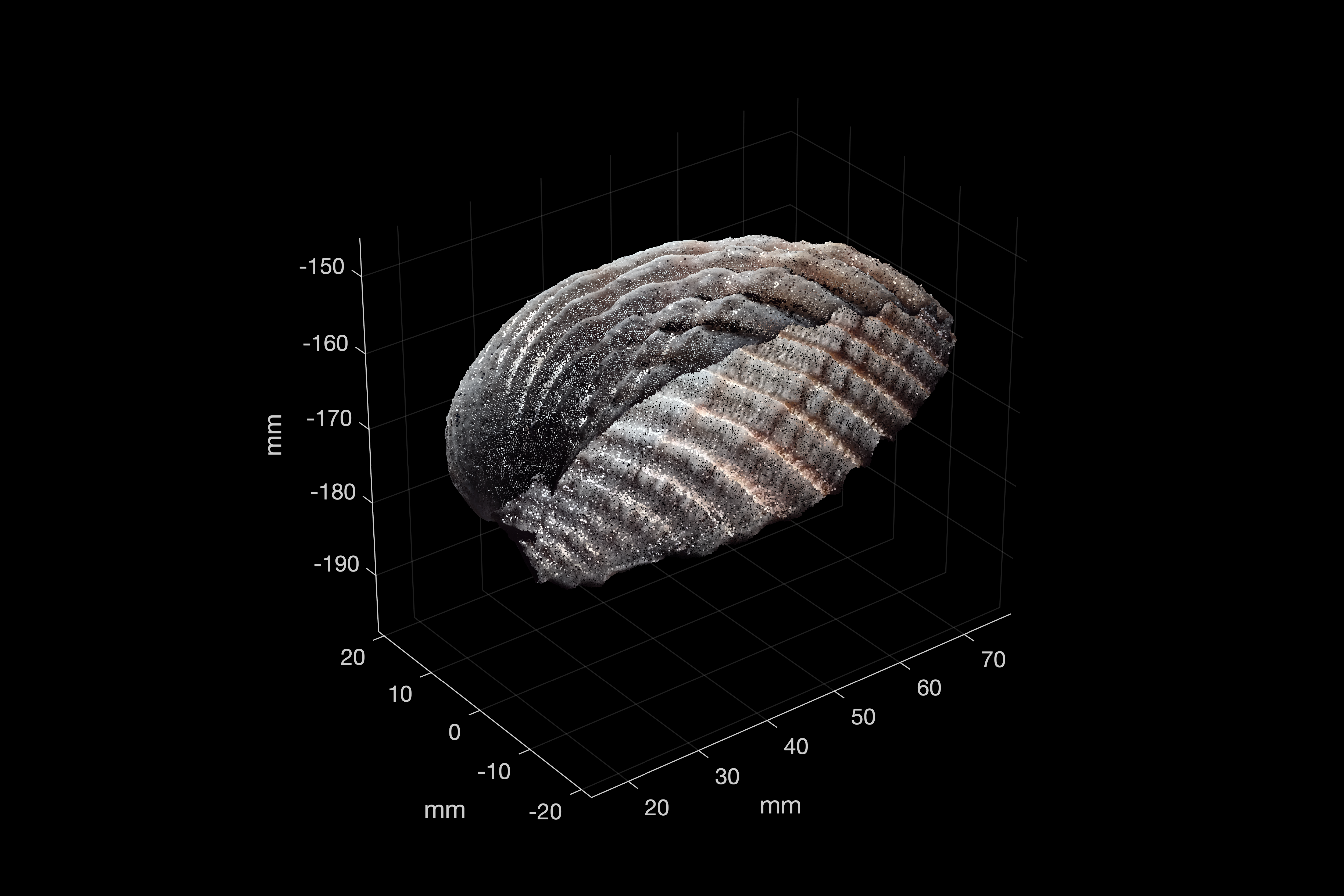
The point cloud object contains 190,436 xyz coordinates of the points in 3D measured by the Depth Camera, the coordinate axes X,Y and Z in millimeters, the RGB color (or texture) in an unsigned integer 8-bit (uint8) format for each point measured by the RGB Camera, and the normal vectors for each point. The grayscal intensity is empty as it was not measured by the scanner. We can display the point cloud using pcshow
figure('Position',[100 800 600 400])
ax = axes('View',[-37.5,30]);
pcshow(pcshellfuse,...
   'AxesVisibility','On',...
   'Parent',ax)
ax.XLabel.String = 'mm';
ax.YLabel.String = 'mm';
ax.ZLabel.String = 'mm';

print -dpng -r600 shellfuse.png
The result is surprisingly good for a fairly inexpensive scanner under 1,000 €. I will work with it a bit more shortly and present it here.