
While I was writing the new book Python Recipes for Earth Sciences, a Python version of my popular textbook MATLAB Recipes for Earth Sciences, difficulties kept cropping up in reproducing the MATLAB graphs. Either it took much longer with Python or the graphics were just less pretty. Of course, it’s up to me, a less experienced Python user, so I invite all Python users to do better!
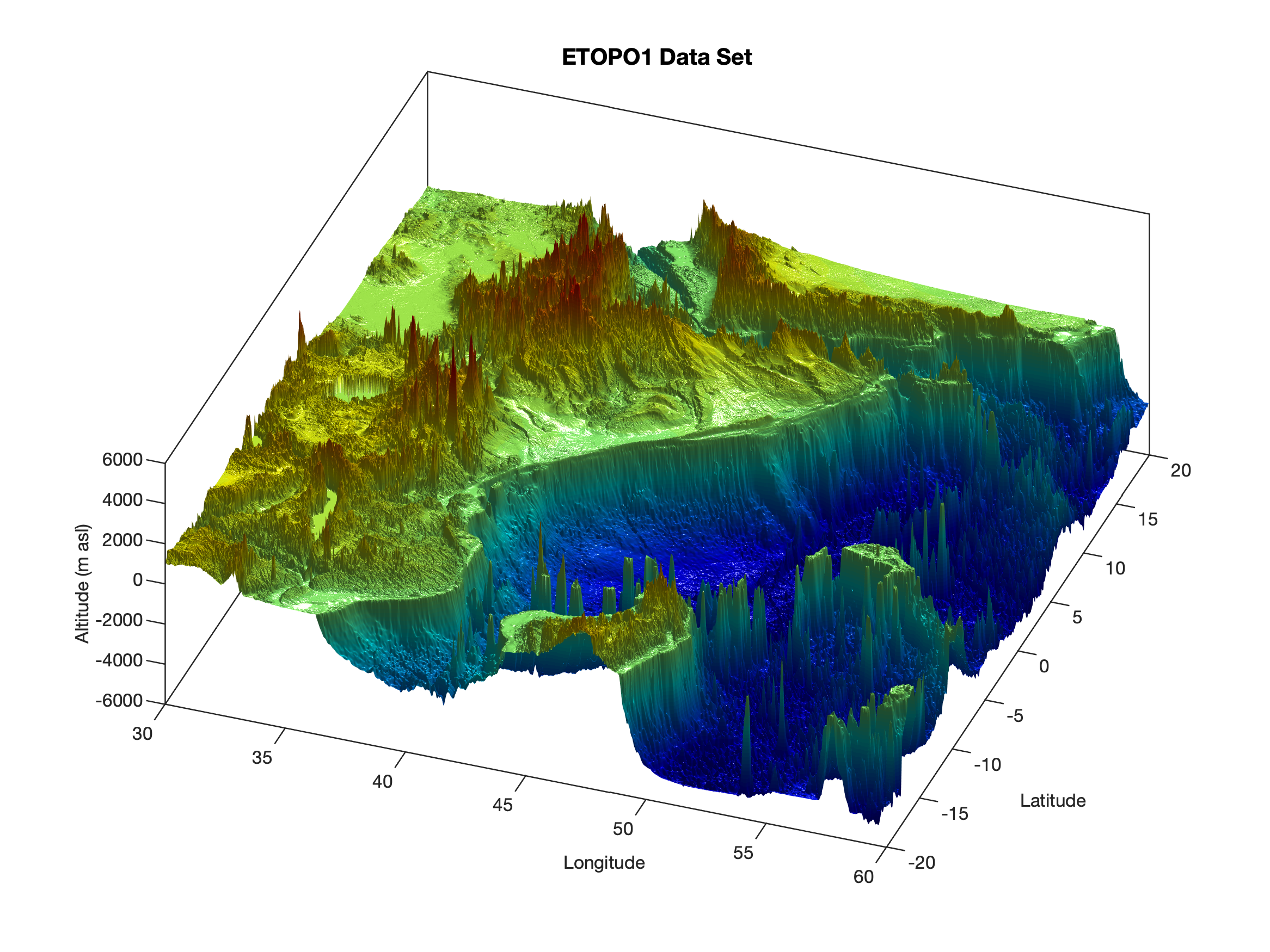
It is about the 3D representation of the The 1 arc-minute global relief model of the Earth’s surface (ETOPO1) data set, which is discussed and visualized in chapter 7.3 of my book. The ETOPO1 data set is a global database of topographic and bathymetric data on a regular 1 arc-minute grid (about 2 km) (Amante and Eakins 2009). Older ETOPO2 and ETOPO5 global relief grids have been superseded but are still available. ETOPO1 is a compilation of data from a variety of sources. It can be downloaded from the NOAA National Centers for Environmental Information (NCEI) webpage. We can download either the whole-world grids, or custom grids for ice surface or bedrock.
The MATLAB code to create the figure and published in the book takes 0.77 s to render and display the graphic on a 16-core Mac Pro (2019) with 96 GB physical memory:
ETOPO1 = load('etopo1_data.txt');
ETOPO1 = flipud(ETOPO1);
ETOPO1(ETOPO1 == -32768) = NaN;
[LON,LAT] = meshgrid(30:1/60:60,-20:1/60:20);

tic

figure('Color',[1 1 1]);
axes('Box','on',...
   'View',[20 60],...
   'LineWidth',0.6,...
   'FontSize',8), hold on
surf(LON,LAT,ETOPO1,...
   'SpecularExponent',20,...
   'FaceLighting','phong',...
   'FaceColor','interp',...
   'EdgeColor','none')
light('Style','local',...
   'Position',[145 70 155801]);
title('ETOPO1 Data Set',...
   'FontSize',10)
xlabel('Longitude',...
   'FontSize',8)
ylabel('Latitude',...
   'FontSize',8)
zlabel('Altitude (m asl)',...
   'FontSize',8)
colormap(jet)

toc

print -dpng -r300 etopo1.png
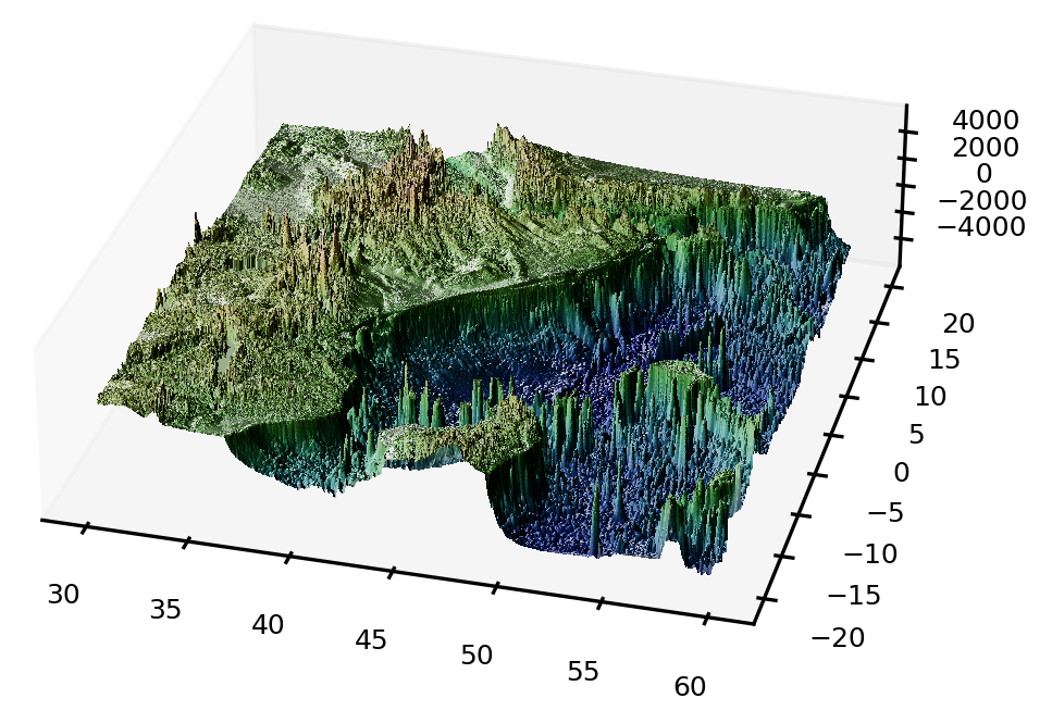
In contrast the Python code below, inspired by a discussion I had on Stackoverflow, takes 121 s to create the graphic on the same computer:
import numpy as np
from matplotlib import cm
import matplotlib.pyplot as plt
from matplotlib.colors import LightSource
import time as time

ETOPO1 = np.loadtxt('etopo1_data.txt')
ETOPO1 = np.flipud(ETOPO1)
lon = np.linspace(30,60,1801)
lat = np.linspace(-20,20,2401)
LON,LAT = np.meshgrid(lon,lat)

starttime = time.time()

plt.figure()
fig, ax2 = plt.subplots(subplot_kw={"projection": "3d"})
ve = 500
ax2.set_box_aspect((1,1,ve/1850))
ls = LightSource(270,45)
rgb = ls.shade(ETOPO1,
cmap=cm.gist_earth,
vert_exag=ve/1850,
blend_mode='hsv')
ax2.plot_surface(LON,LAT,ETOPO1,
rstride=1,
cstride=1,
linewidth=0,
facecolors=rgb,
antialiased=False,
shade=True)
ax2.tick_params(axis='both',
labelsize=6)
ax2.view_init(30,15-90)
ax2.grid(False)

endtime = time.time()

plt.savefig('etopo1_python.png',dpi=300)
plt.show()

print(endtime-starttime)
Can you do it better? Then send me an email with your code and a 300 dpi version of the graphic.
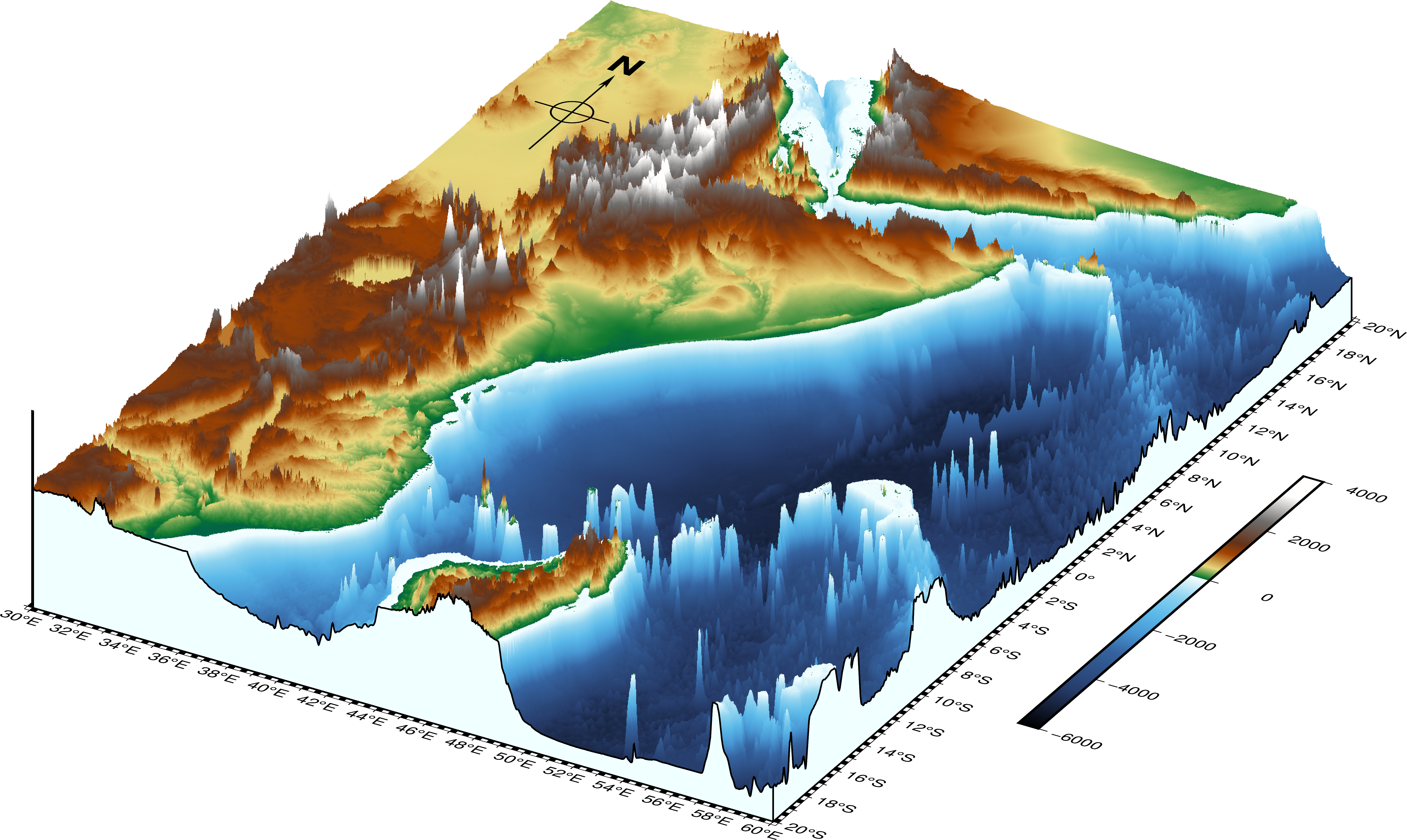
My colleague Norbert Marwan sent me a script which makes use of the excellent PyGMT package. Here is a slightly modified version of Norbert’s script, which is much faster than the script to create the graphics using the Matplotlib package and the output looks much more beautiful:
import numpy as np
import pygmt as pygmt
import xarray as xr
from matplotlib import cm
import matplotlib.pyplot as plt
from matplotlib.colors import LightSource

ETOPO1 = np.loadtxt('etopo1_data.txt')
ETOPO1 = np.flipud(ETOPO1)

lon = np.linspace(30,60,1801)
lat = np.linspace(-20,20,2401)
LON,LAT = np.meshgrid(lon,lat)

ds = xr.DataArray(data=ETOPO1,
    dims=['lat','lon'],
    coords={'lat':lat,'lon':lon})
frame = ['xa1f0.25','ya1f0.25','wSEnZ']
pygmt.makecpt(
    cmap='geo',
    series=f'-6000/4000/10',
    continuous=True)
fig = pygmt.Figure()
fig.grdview(grid=ds,
    perspective=[150,30],
    frame=frame,
    projection='M15c',
    zsize='4c',
    surftype='i',
    plane='-6000+gazure',
    shading=0)
fig.basemap(
    perspective=True,
    rose='jTL+w3c+l+o-2c/-1c')
fig.colorbar(perspective=True,
    position='JMR+o2c/0c+w10c',
    frame=['a2000'])
fig.show()
References
Amante C, Eakins BW (2009) ETOPO1 1 Arc-Minute Global Relief Model: Procedures, Data Sources and Analysis. NOAA Technical Memorandum NESDIS NGDC-24
Trauth, M.H. (2021) MATLAB Recipes for Earth Sciences – Fifth Edition. Springer International Publishing, ~500 p., Supplementary Electronic Material, Hardcover, ISBN: 978-3-030-38440-1.