
If you want to write code for geoscientific data analysis independent of the programming language, a comparison of the syntax helps. And there are many similarities, not least because the languages inspire each other, even in the names of functions, which makes trilingual coding easy. Here is an example.
MATLAB, Python, and Julia share common roots in that they rely on the same standardized vectorized computations included in open-source FORTRAN libraries LAPACK and BLAS. This continues one level up, as more advanced algorithms such as the FFT are also standardized and, if programmed correctly and free of floating point errors, should give the same result. At this level, algorithms in MATLAB are often not visible, in contrast to open-source Python and Julia, as you can in an excellent Julia example by Bogumił Kamiński on his blog.
In MATLAB these functions are called “built-in functions”, but first, you can easily check the correctness of the algorithms on standardized examples, as it is done in the MRES book in numerous places. Secondly, MathWorks offers a warranty, the possibility of certification of code and comprehensive information from MATLAB support. On the next higher level, MATLAB, like Python and Julia, is also open source: the code of the FFT-based periodogram, for example, can be viewed by typing “edit periodogram” in the Command Window.
Most of these functions, such as periodogram, are not included in the standard MATLAB, Python, or Julia package. They are part of toolboxes (MATLAB) or packages (Python, Julia). In MATLAB, there are ~90 toolboxes offered by the vendor MathWorks, and a large number of user-contributed toolboxes, many of which are offered through the File Exchange or personal websites like this blog. Python packages are listed in the Python Package Index and Julia packages are collected in the General Registry.
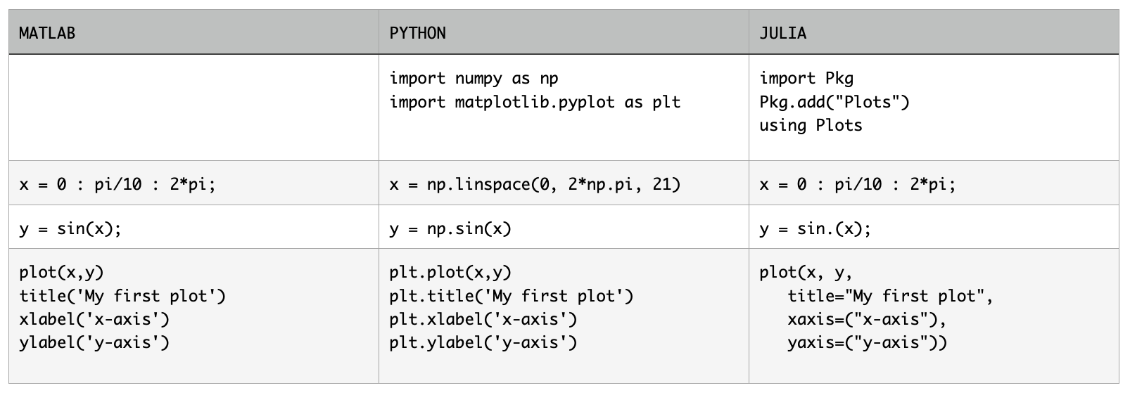
Having said that let us have a look at a simple coding project first, with MATLAB, then Python and Julia. One of the first differences between the three languages is clearing the workspace, which Python and Julia don’t do with a simple command like clear in MATLAB. There are many forum posts about this from former MATLAB users who switch to Python or Julia: where is the clear? We then create a simple vector x, calculate the sine of x and create a xy plot:
clear
x= 0 : pi/10 : 2*pi;
y = sin(x);

plot(x,y)
title('My first plot')
xlabel('x-axis')
ylabel('y-axis')
You can also use
x = linspace(0,2*pi,21);
instead, similar to the function used in the Python code. Interestingly, the linspace function has recently been removed from Julia and therefore range has to be used instead, a function that also exists in Python but with a different functionality. Typing whos in the MATLAB Command Window lists the variables in the workspace:
Name   Size   Bytes  Class   Attributes

x      1x21   168    double
y      1x21   168    double
In Python, similar to Julia, we have to import NumPy and Matplotlib, two packages with MATLAB-style functions for scientific computing and visualization. We import these packages and assign abbreviations like np and plt to them, so that we can identify the functions used from those packages in the code; it is not recommended to import the packages as *, as it is sometimes done for convenience by MATLAB switchers.
import numpy as np
import matplotlib.pyplot as plt
We then create x using linspace and calculate y as the sine of x. We then plot the result.
x = np.linspace(0, 2*np.pi, 21)
y = np.sin(x)

plt.plot(x,y)
plt.title('My first plot')
plt.xlabel('x-axis')
plt.ylabel('y-axis')
Using np.who() lists the NumPy arrays in the workspace:
Name    Shape    Bytes    Type
===============================================

x       21       168      float64
y       21       168      float64

Upper bound on total bytes = 336
Alternatively, whos lists everything in the workspace, including the imported packages. The syntax of Julia is somewhat more similar to that of MATLAB, which seems to be intentional and has been described many times. Again we have to import packages, such as the one to create plots. Here, Pkg is the builting package manager that handles operations such as installating, updating and removing packages. Here, we use the Plots package listed in the General Registry.
import Pkg
Pkg.add("Plots")
using Plots

x = 0 : pi/10 : 2*pi;
y = sin.(x);

plot(x, y1,
title="My first plot",
xaxis=("x-axis"),
yaxis=("y-axis"))
The function whos() is another example of a function that has been removed from Julia (version 1.0 onward). Instead we can use varinfo() to get
name                     size  summary
–––––––––––––––––––––––––––––––––––––––––––––––––––
Base                           Module
Core                           Module
InteractiveUtils  260.128 KiB  Module
Main                           Module
ans                27.720 KiB  Plots.Plot{Plots....
x                    48 bytes  21-element StepRa...
y                   208 bytes  21-element Vector...
All three scripts provide comparable plots with titles and axis labels. In MATLAB the Live Editor and in Python the Jupyter Notebook furthermore help to provide an appealing design with designed headings, comments and code, together with embedded graphs, which can be exported as PDF.
Download the MATLAB, Python and Julia examples. Please send comments, corrections, and additions via email to trauth@geo.uni-potsdam.de.