
 Are you still buying CDs, or you just stream your music? Or, possibly you just got a vinyl record and wonder why it is gaining popularity again? A short lecture about sampling frequencies, aliasing and the Nyquist frequency with MATLAB examples.
One of the most common effects of sampling is aliasing. This term refers to the misinterpretation of a sine wave with a frequency f, which is higher than the sampling frequency fs, as a sine wave with an alias frequency fa, which is lower than the sampling frequency. Aliasing is also known as a stroboscopic effect or a wagon wheel effect in human visual perception. This effect means that if objects that are rotating quickly and smoothly at a high frequency, such as the wheels of a wagon, are recorded with a video camera, operating at a sampling frequency of 24 frames per second, they will appear to be circling backward at a lower frequency. We can calculate fa using
![]()
where round stands for rounding to the nearest integer. We can use this as our first MATLAB example, demonstrating the effect of sampling a sinusoidal signal with a frequency f at a sampling rate of fs that is too low to describe the signal accurately. As an example, we generate a sine wave with a frequency of f=1/2=0.5 (corresponding to a period of 2) (Trauth 2020) using
t = 0 : 0.1 : 15; t = t';
x1 = sin(2*pi*t/2);
If this signal, originally sampled with a frequency of fs=1/0.1=10, is sampled with a frequency that is too low, e.g. fs=1/1.6=0.6250, we generate an alias frequency of fa=1/8=0.1250, as we can calculate with the formula from above:
fa = abs(0.5 - 0.6250 * round(0.5/0.6250))
which yields
fa =
    0.1250
We can demonstrate the aliasing effect with this example, if we actually sample the signal with the lower sampling rate of fs=0.6250,
ts = 0 : 1.6 : 15; ts = ts';
x2 = interp1(t,x1,ts,'linear','extrap');
shift the resulting signal by 3.5 to align it with the original signal
x3 = sin(2*pi*t*fa + 2*pi*3.5);
and display the result.
figure('Position',[100 1000 600 300])
axes('Position',[0.1 0.2 0.8 0.7],...
  'Box','On',...
  'LineWidth',1,...
  'FontSize',14,...
  'YLim',[-1.2 1.2])
hold on
line(t,x1,...
  'Color',[0 0.4471 0.7412],...
  'LineWidth',1.5)
s1 = stem(ts,x2,...
  'Color',[0.8510 0.3255 0.0980],...
  'LineWidth',1.5,...
  'Marker','o',...
  'MarkerSize',14);
line(t,x3,...
  'Color',[0.9294 0.6941 0.1255],...
  'LineWidth',1.5)
xlabel('Time')
s1.BaseLine.LineStyle = ':';
s1.BaseLine.LineWidth = 1;
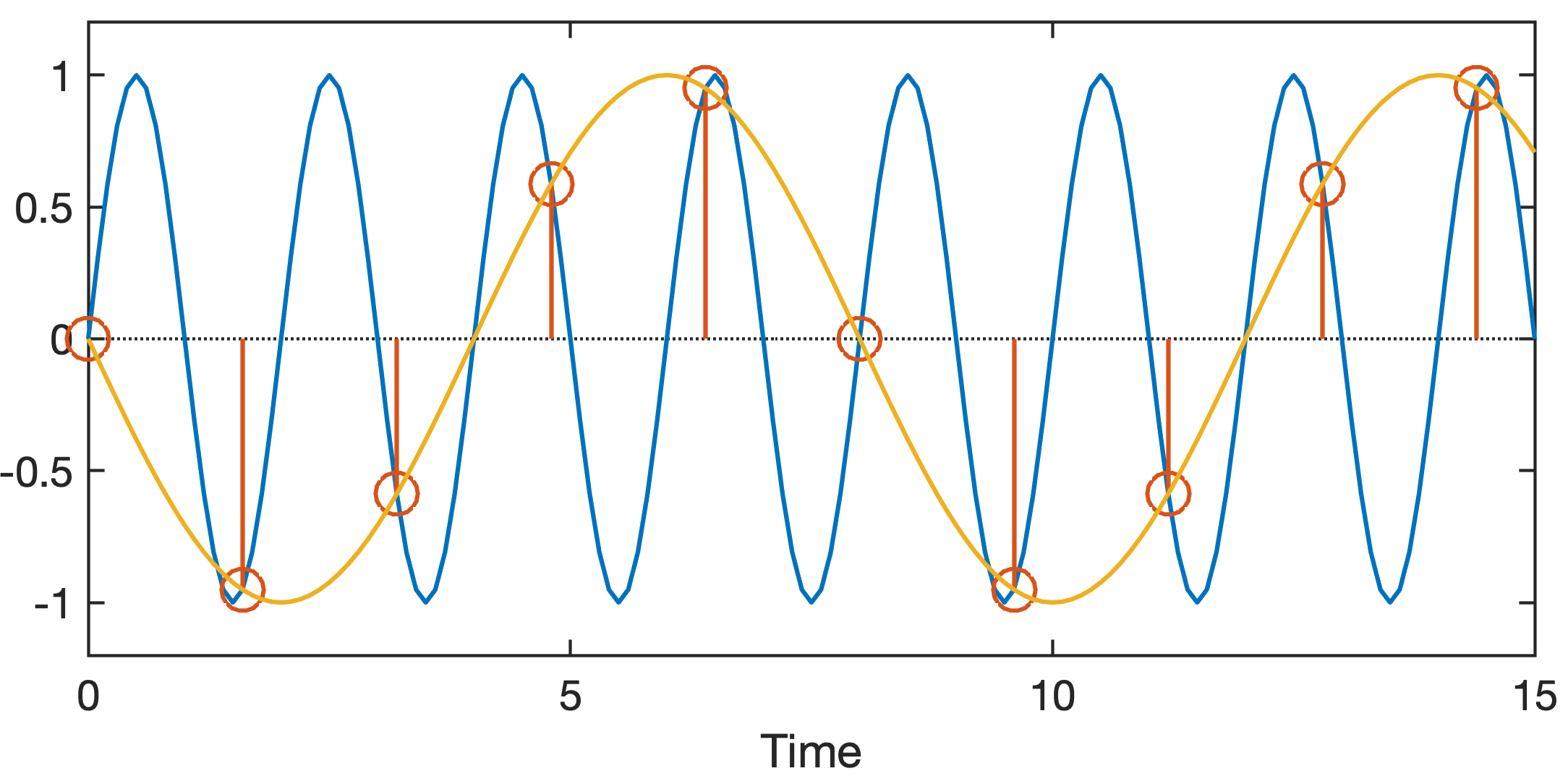
The graphic illustration shows that the signal with the frequency f=0.5 (corresponding to a period of 1/0.5=2) (blue line), sampled with a low sampling frequency fs=0.3125 (corresponding to a sampling interval of 1/0.3125=3.2) (red stems and circles), produces a signal with a lower aliasing frequency fa=0.1250 (corresponding to a alias period of 1/0.1250=8) (yellow line).
The effect of aliasing can be avoided by applying the Nyquist–Shannon sampling theorem, according to which the sampling frequency fs must be at least twice the frequency of interest. Spectral representations of signals are therefore shown at half the sampling frequency (fs/2), which is called the Nyquist frequency fNyq and was defined by the American mathematician Claude Elwood Shannon and named after the Swedish-American electrical engineer Harry Nyquist. Compact discs (CDs) provide a good example of an application of the Nyquist-Shannon sampling theorem: CDs are sampled at frequencies of 44,100 Hz (Hertz, where 1 Hz=1 cycle per second) but the corresponding Nyquist frequency is 22,050 Hz, which is the highest frequency a CD player can theoretically produce. The performance limitations of anti-alias filters used by CD players further reduce the frequency band and result in a cutoff frequency of around 20,050 Hz, which is the true upper-frequency limit of a CD player.
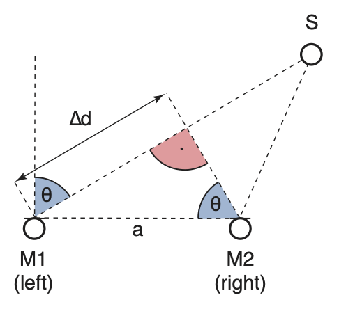
The limitation of the frequency band of CDs to 20,050 Hz in contrast to vinyl records is often brought up as a reason for the better sound of vinyl and controversially discussed among supporters of one or the other technology. This overlooks another difference, the poorer spatial reproduction of music on CDs due to the restriction to frequencies <20.050 Hz. The following exercise will demonstrate the use of an active method for localizing a sound source by determining its distance from the receiver (e.g. Weinzierl 2008, Mugagga and Winberg 2015). For this, we use a simple stereo microphone, i.e. two separate receivers or microphones M1 and M2, set up a specific distance a apart. The sound waves emitted by a source S reach the two microphones at different times unless S is on the perpendicular bisector of the line between M1 and M2. If we clap our hands as a sound source, for example, we can then use the measured difference in travel time and the known velocity of sound in air at 20°C of ~340 m/s to calculate the difference in the travel distances Δd between the sound source and the two microphones. The arcsine of the ratio of Δd to the distance between the microphones a yields the direction of the sound source θ.
This exercise uses a Logitech C930e webcam with two electret condenser bidirectional microphones. The camera’s datasheet indicates a frequency range for the microphones of 100–7,000 Hz and a sensitivity of –45±3 dB. Bidirectional microphones pick up sound waves well from either the back or the front and reject sound coming from the sides. This makes them useful for localizing sound by time-of-arrival stereophony, using devices such as webcams or smartphones that have small distances between the two receivers. In our example, the distance between the two microphones M1 and M2 is ~7.57 cm according to the information provided by All About Circuits, which is an independent online community for electrical engineers. This results in a maximum travel time difference of 0.00022 s if the direction of the sound source is θ=–90° or θ=+90°.
The human ear is able to hear sounds with frequencies between 20 Hz and 20 kHz, corresponding to periods of between 0.05 s and 0.05 ms, but differences in travel time of 0.01–0.02 ms to determine the direction to a sound source, which is enough to determine the direction with an accuracy of 1° (e.g. Ellermeier and Hellbrück 2008). To digitally record such a small difference in travel time would require a sampling frequency of 50–100 kHz. Assuming that M1 represents a person’s left ear and M2 the right ear and that their separation is 21.5 cm, then a sound source in line with the ears would yield the maximum difference in arrival times (~0.73 ms for a sound velocity in the air of 340 m/s). Such travel time differences cannot be reproduced by a compact disc (CD) due to their limited frequency response (between 20 Hz–20 kHz), which severely restricts their stereophonic capabilities compared to analog vinyl records, which have a frequency response of at least 50 kHz, and theoretically even as high as 100 kHz (depending on the cartridge and stylus profile). Even though the human ear is not able to hear frequencies above 20 kHz, audio information in the 20–25 kHz range certainly contributes to the stereophonic sound source location.
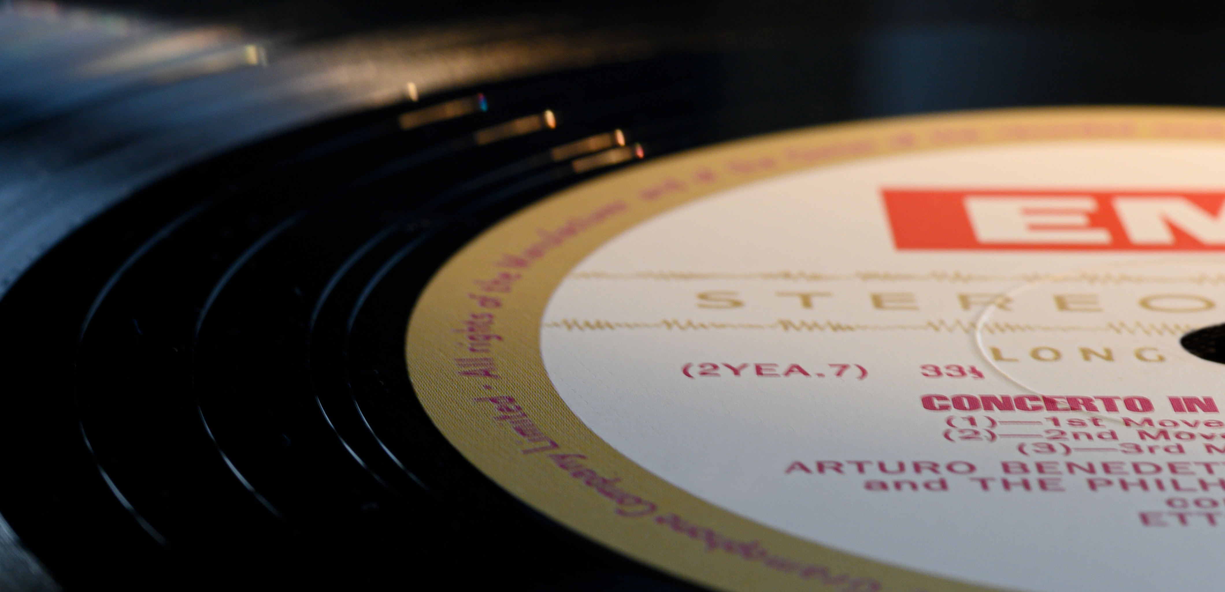
This phenomenon can be easily verified by stereo recordings of classical music or acoustic jazz from the late 50s (after the invention of the Full Frequency Stereophonic Sound) and 60s, which did not fall victim to digital processing of the late 70s and after, but were pressed on vinyl largely unaltered. A nice example is the 1957 EMI recording of Maurice Ravel’s Piano Concerto in G major by Arturo Benedetti Michelangeli with the Philharmonia Orchestra conducted by Ettore Gracis, available both on vinyl and compact disc. This recording has a wonderful three-dimensional sound, with the grand piano clearly in front of the orchestra, while the CD version of the same recording sounds flat.
References
Muggaga PKB, Winberg S (2015) Sound Source Localisation on Android Smartphones: A first step to using smartphones as auditory sensors for training A.I systems with Big Data. IEEE AFRICON 2015, 1–5
Ellermeier W, Hellbrück J (2008) Hören – Psychoakustik – Audiologie, in Weinzierl S, Handbuch der Audiotechnik. Springer, Berlin Heidelberg New York, 42–85
Trauth MH (2020) MATLAB Recipes for Earth Sciences – Fifth Edition. Springer, Berlin Heidelberg New YorkWeinzierl S (2008) Handbuch der Audiotechnik. Springer, Berlin Heidelberg New York
Trauth, M.H. (2021) Signal and Noise in Geosciences, MATLAB Recipes for Data Acquisition in Earth Sciences. Springer International Publishing.
Weinzierl S (2008) Handbuch der Audiotechnik. Springer, Berlin Heidelberg New York