
The XRF data from our sediment cores from the Chew Bahir show dramatic jumps. If we analyze them statistically, the results will be affected by these changes in the mean. That’s why I was looking for ways to remove them. Here are two of these ways to remove jumps.
First, let us generate synthetic data, a simple sine wave without noise, and add two jumps up and down.
clear, clc, close all
t = 0 : 0.1 : 10*pi;
x1 = sin(t);
x1(1,131:315) = x1(1,131:315) + 5;
x1(1,170:315) = x1(1,170:315) - 10;
The first way of removing jumps is to calculate the 1st derivative with diff, with jumps indicated by outliers to be removed e.g. by using the function filloutliers, introduced in R2017a. Then, we integrate the time series and add one single NaN at the end of the time series that got lost while using diff.
x2 = diff(x1);
x3 = filloutliers(x2,'pchip');
x4 = cumsum(x3);
x4(end+1) = NaN;

figure('Position',[100 100 800 1000])
axes('Position',[0.1 0.8 0.8 0.15])
plot(t,x1), grid
title('Original Data with Jumps')
axes('Position',[0.1 0.6 0.8 0.15])
plot(t(1:end-1),x2), grid
title('1st Derivative')
axes('Position',[0.1 0.4 0.8 0.15])
plot(t(1:end-1),x3), grid
title('1st Derivative, Outliers removed')
axes('Position',[0.1 0.2 0.8 0.15])
plot(t,x1,t,x4), grid
title('Integrated Signal')
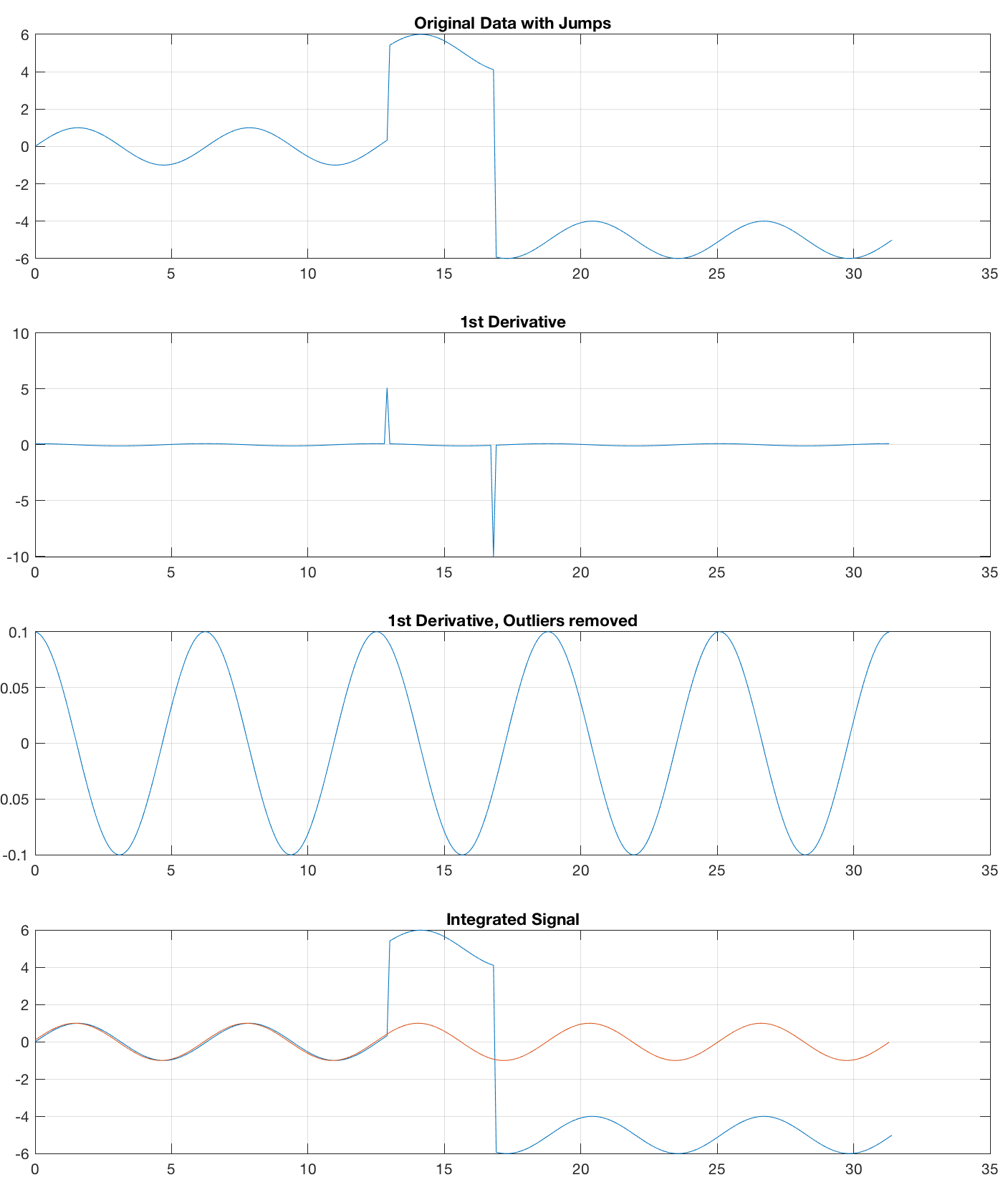
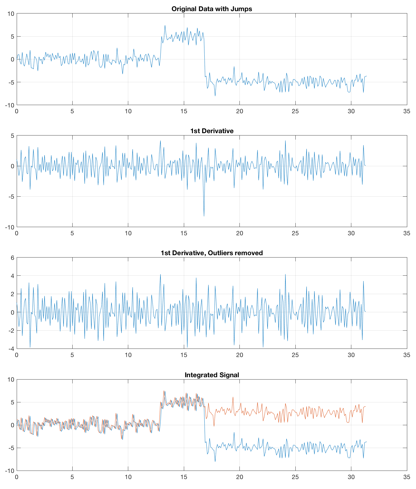
This works fine for the noisefree sine wave but fails to remove jumps from noise, created with x1 = randn(size(t));
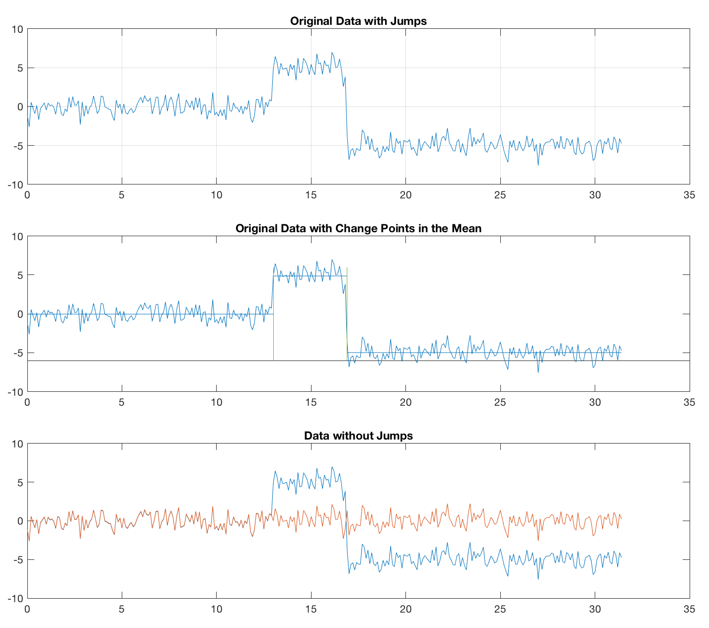
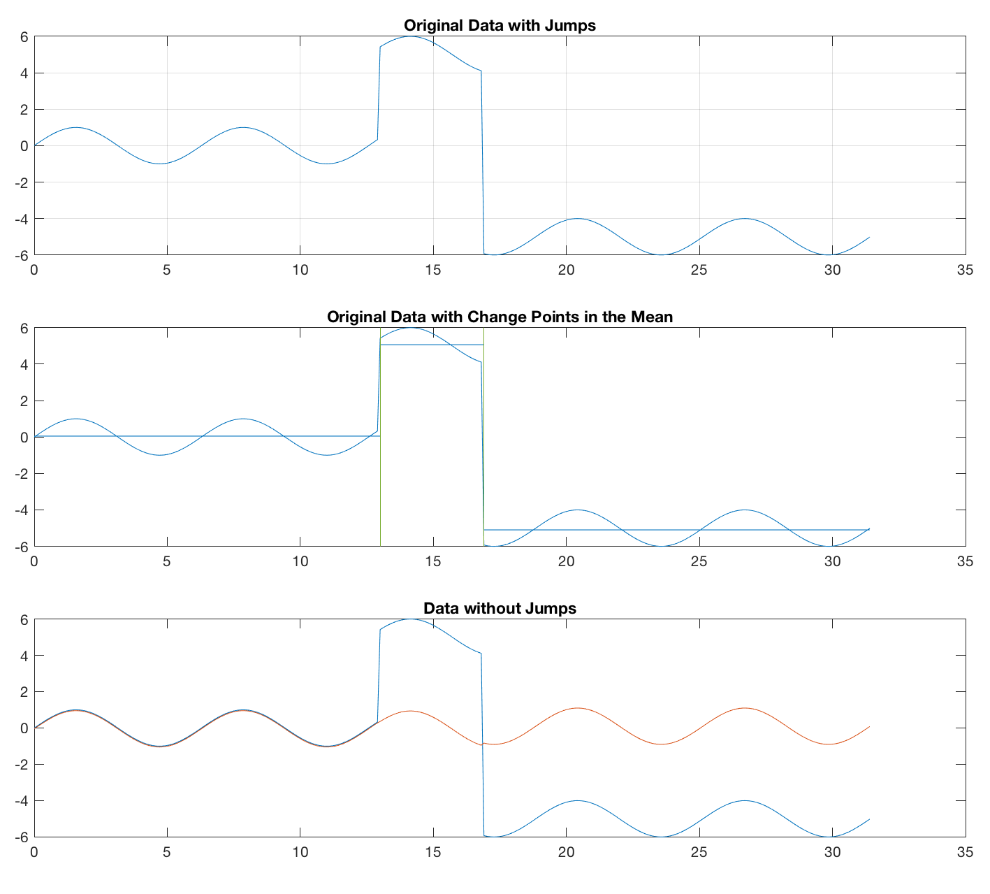
Therefore, I tried an alternative approach, using the function findchangepts, contained in the Signal Processing Toolbox and introduced in R2016. The function has been discussed to find change points in an earlier post. We use the function, define the number of change points we expect, and remove the mean (alternatively the median) from the segments between the change points. This approach seems to work fine for both sine waves and noise.
clear x2 x3 x4

maxnumchg = 2;
[ipoint,residual] = findchangepts(x1,...
   'MaxNumChanges',maxnumchg);
m(1) = mean(x1(1:ipoint(1)));
for i = 1 : length(ipoint)-1
    m(i+1) = mean(x1(ipoint(i):ipoint(i+1)));
end
m(length(ipoint)+1) = mean(x1(ipoint(i+1):end));

x2 = zeros(size(x1));
x2(1:ipoint(1)) = x1(1:ipoint(1)) - m(1);
for i = 1 : length(ipoint)-1
    x2(ipoint(i):ipoint(i+1)) = ...
    x1(ipoint(i):ipoint(i+1)) - m(2);
end
x2(ipoint(i+1):end) = x1(ipoint(i+1):end) - m(end);

figure('Position',[100 100 800 1000])
axes('Position',[0.1 0.8 0.8 0.15])
plot(t,x1), grid, title('Original Data with Jumps')
axes('Position',[0.1 0.6 0.8 0.15],...
    'XLim',[0 35],'Box','On'), hold on
line(t,x1)
line([0 t(ipoint(1))],[m(1) m(1)])
for i = 1 : length(ipoint)-1
    line([t(ipoint(i)) t(ipoint(i+1))],...
    [m(i+1) m(i+1)])
end
line([t(ipoint(length(ipoint))) t(end)],...
    [m(end) m(end)])
stem(t(ipoint),6*ones(size(t(ipoint))),...
    'Marker','none',...
    'Color',[0.4667 0.6745 0.1882],...
    'BaseValue',-6)
title('Original Data with Change Points')
axes('Position',[0.1 0.4 0.8 0.15])
plot(t,x1,t,x2)
title('Data without Jumps')
This method also works fine, of course, for the sine wave.
You can download the full code of both experiments using this link.