
MATLAB is a great tool to simulate error propagation. As an example we will use the software to estimate the uncertainty in the difference between the measures of two quantities A and B, based on their individual uncertainties σA and σB. The experiment shows the error of differences in case the errors are either dependent or independent of each other.
We first clear the workspace, the Command Window and close all Figure windows.
clear, clc, close all
samplesize = 100000000;
To calculate the differences between A and B, and the error of this difference, we use two Gaussian distributions A and B, with mean values of 6.3 and 3.4, i.e. with a difference of 6.3-3.4 = 2.9, and standard deviations of 1.2 and 1.5, respectively. We calculate the difference between the mean values of the two distributions on the assumption that the two distributions are dependent of each other. According to the article about the propagation of uncertainty of Wikipedia, the function then is
f = aA – bB
which yields
f = 6.3 – 3.4 = 2.9
with the real variables A, B with standard deviations σA and σB, and covariance σAB and exactly known real-valued constants a, b. Then the variance is
σf2 = a2σA2 + b2σB2 – 2abσAB
which yields
σf2 = 1.52 + 1.22 – 2 · 1.5 · 1.2 = 0.09
and therefore
σf = 0.3
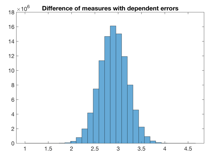
which is the error of the difference of two measurements for perfectly dependent errors. Using a MATLAB experiment, we use the same set of random numbers r to add uncertainty to the data.
rng(0)
r = randn(samplesize,1);
age1 = 3.4 + 1.2*r;
age2 = 6.3 + 1.5*r;
dage = age2-age1;

figure(...
 'Position',[200 200 600 400],...
 'Color',[1 1 1]);
axes(...
 'Box','on',...
 'Units','Centimeters',...
 'LineWidth',0.6,...
 'FontName','Helvetica',...
 'FontSize',14); hold on
histogram(dage,30)

mean(dage)
std(dage)
which yields
ans = 2.9000
and
ans = 0.3000
for the difference in the mean and its error.
Now we run the same experiment but now the two measurements are independent from each other. Then the covariance term is zero and
σf2 = a2σA2 + b2σB2 – 2abσAB2
yields
σf2 = 1.52 + 1.22 – 0 = 3.6900
and therefore
σf = 1.9200
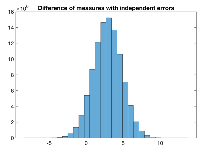
which is the error of the difference of two measurements for perfectly independent errors. Using a MATLAB experiment, we use the different sets of random numbers to add uncertainty to the data.
rng(0)
age1 = 3.4 + 1.2*randn(samplesize,1);
age2 = 6.3 + 1.5*randn(samplesize,1);
dage = age2-age1;

figure(...
 'Position',[200 800 600 400],...
 'Color',[1 1 1]);
axes(...
 'Box','on',...
 'Units','Centimeters',...
 'LineWidth',0.6,...
 'FontName','Helvetica',...
 'FontSize',14); hold on
histogram(dage,30)

mean(dage)
std(dage)
which yields
ans = 2.8998
and
ans = 1.9207
for the approximately the difference in the mean and its error. The small deviation from the exact values used to create the data is due to the limited sample size.
Reference
Tayler, J.R. 1997, An introduction to error analysis – the study of uncertainties in physical measurements, 2nd edition. University Science Books, 527 pages.