
In a series of blog posts, I will tell you a little about how I teach computational geosciences with MATLAB. On the second half of day 2 of the one-week course I teach bivariate statistics.
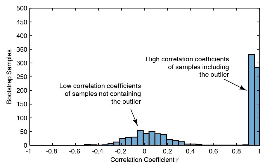
First I explain students how to compute a correlation coefficient. We start with the very popular Pearson correlation coefficient, discuss its weaknesses, before I introduce alternative correlation coeffients explained in an earlier post. Then bootstrapping is introduced to detect outliers in bivariate data. The second part of the course on bivariate statistics is about regression. After introducing the classic linear regression and common mistakes of its use, I discuss a selection of examples of use and misuse of the method in prediction.
As an example we discuss a paper by Rahmstorf (Science 2007). The paper tries to build a linear model for predicting future sea level rise from historical data of the rate of sea-level rise and air temperature. Nothing wrong with the regression analysis itself but the pretreatment of the data, as said in the caption of Figure 2, changes the significance of the result, as said in a comment by Holgate et al. (Science 2007): “Data were binned in 5-year averages to illustrate this correlation” (Rahmstorf, Science 2007).
References
Rahmstorf, S. (2007) A Semi-Empirical Approach to Projecting Future Sea-Level Rise. Science, 315, 368-370.
Holgate, S. et al. (2007) Comment on “A Semi-Empirical Approach to Projecting Future Sea-Level Rise”. Science, 317, 1866.