Stratigraphic Correlation of Multiple Sediment Cores Using MATLAB, Part 2

In geological drilling projects, two or more parallel cores often collected in order to compensate for core losses during drilling by overlapping sequences. Correlation of the core is a time-consuming and complex process that is usually done by very experienced geologists. Yesterday I posted the script for manual correlation of core records based on visual inspection of the record of sediment physical properties. This post explains how to use dynamic time warping for automated correlation of cores.

Dynamic time warping uses similarities for matching time series. The method is, as an example, widely used in speech recognition, where different speaking speeds hamper the correlation of time series. First, we have to define the segment of the core to be correlated, defined by the mimimum and maximum x-value, XMin and XMax, which could be depth below surface in meters.

clear, clc, close all
XMin = 0;
XMax = 30;

Then import the sample data from files data_1.txt and data_2.txt.

data1 = load('data_1.txt');
data2 = load('data_2.txt');

We can then eliminate duplicate data points by typing

for i = 1:size(data1)-1
   if data1(i,1) == data1(i+1,1)
      data1(i,1) = NaN;
   end
end
data1(isnan(data1(:,1))==1,:) = [];
for i = 1:size(data2)-1
   if data2(i,1) == data2(i+1,1)
      data2(i,1) = NaN;
   end
end
data2(isnan(data2(:,1))==1,:) = [];

Define segment to be correlated:

data1 = data1(data1(:,1)>XMin & data1(:,1)<XMax,:);
data2 = data2(data2(:,1)>XMin & data2(:,1)<XMax,:);

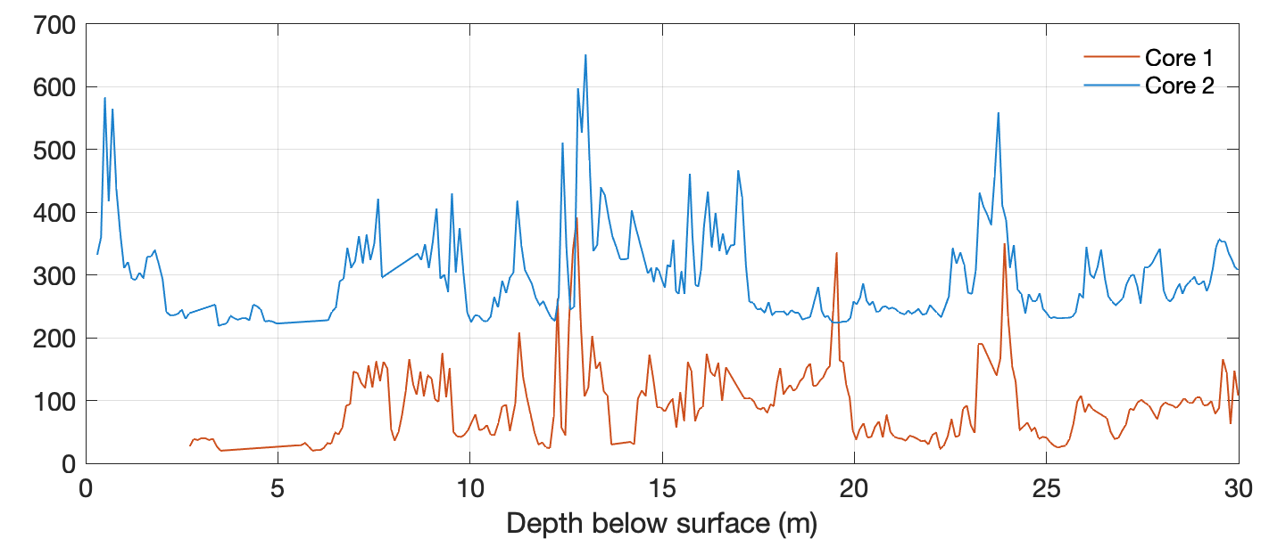
Display the data using:

figure('Position',[50 950 800 300])
axes('Box','On',...
    'XGrid','On',...
    'YGrid','On',...
    'YLim',[0 700]), hold on
line(data1(:,1),data1(:,2),...
    'Color',[0.8 0.3 0.1])
line(data2(:,1),data2(:,2)+200,...
    'Color',[0.1 0.5 0.8])
xlabel('Depth below surface (m)')
legend('Core 1','Core 2')
legend('boxoff')

We use the function dtw from the Signal Processing Toolbox to perform dynamic time warping:

maxsamp = 100;
metric = 'euclidean';
[dist,iydata2,ixdata1] = ...
     dtw(data2(:,2),data1(:,2),maxsamp,metric);

We then display the aligned time series. The max value in ixdata1 is the length of data1 and the max value in iydata2 is the length of data2. We can therefore plot the data in data1 and data2 over the index ixdata1 and ixdata2. The index values ixdata1 and iydata2 are integer values from 1 to length(data1) and 1 to length(data2), but there are duplicate int values due to the introduction of repeated values of data1 and data2.

figure('Position',[50 550 800 300])
axes('Box','On',...
    'XGrid','On',...
    'YGrid','On',...
    'YLim',[0 700]), hold on
line(iydata2,data1(ixdata1,2),...
    'Color',[0.8 0.3 0.1])
line(iydata2,data2(iydata2,2)+200,...
    'Color',[0.1 0.5 0.8])
xlabel('Index')
legend('Core 1','Core 2')
legend('boxoff')

We can also display the index of core 1 and 2 in a xy plot.

figure('Position',[900 850 400 400])
axes('Box','On',...
    'XGrid','On',...
    'YGrid','On'), hold on
line(ixdata1,iydata2,...
    'Color',[0.8 0.3 0.1])
line([ixdata1(1) ixdata1(end)],...
     [iydata2(1) iydata2(end)],...
    'Color','k',...
    'LineStyle',':')
xlabel('Index Core 1')
ylabel('Index Core 2')

We then create new data array of aligned data values.

clear data1i data2i
data1i(:,1) = iydata2;
data1i(:,2) = data1(ixdata1,2);
data2i(:,1) = iydata2;
data2i(:,2) = data2(iydata2,2);

And then we again display the results.

figure('Position',[50 150 800 300])
axes('Box','On',...
    'XGrid','On',...
    'YGrid','On',...
    'YLim',[0 700]), hold on
line(data1i(:,1),data1i(:,2),...
    'Color',[0.8 0.3 0.1])
line(data2i(:,1),data2i(:,2)+200,...
    'Color',[0.1 0.5 0.8])
xlabel('Index')
legend('Core 1','Core 2')
legend('boxoff')

Remove duplicate values after dynamic time warping.

for i = 1:length(data1i)-1
    if data1i(i,1) == data1i(i+1,1)
        data1i(i,:) = NaN;
    end
end
data1i(isnan(data1i(:,1))==1,:) = [];
for i = 1:length(data2i)-1
    if data2i(i,1) == data2i(i+1,1)
        data2i(i,:) = NaN;
    end
end
data2i(isnan(data2i(:,1))==1,:) = [];

Interpolate the data to the same evenly-spaced time axes. It is important to check the resolution of the new time vector. In our example we get about the same number of data points as in the raw data.

clear data1i_int data2i_int
data1i(:,1) = max(data1(:,1))*data1i(:,1)/ ...
    length(data1i(:,1));
data1i_int(:,1) = 0:mean(diff(data1(:,1))):...
    max(data1(:,1));
data1i_int(:,2) = interp1(data1i(:,1),...
    data1i(:,2),data1i_int(:,1),...
    'linear','extrap');
data2i(:,1) = max(data2(:,1))*data2i(:,1)/ ...
    length(data2i(:,1));
data2i_int(:,1) = data1i_int(:,1);
data2i_int(:,2) = interp1(data2i(:,1),...
    data2i(:,2),data2i_int(:,1),...
    'linear','extrap');

Display the results.

figure('Position',[50 150 800 300])
axes('Box','On',...
    'XGrid','On',...
    'YGrid','On',...
    'YLim',[0 700]), hold on
line(data1i_int(:,1),data1i_int(:,2),...
    'Color',[0.8 0.3 0.1])
line(data2i_int(:,1),data2i_int(:,2)+200,...
    'Color',[0.1 0.5 0.8])
xlabel('Composite depth below surface (m)')
legend('Core 1','Core 2')
legend('boxoff')

We can then calculate the piecewise cross correlation over a window of length w.

w = 50;
hwait = waitbar(0,'Please wait ...');
for i = w/2+1:length(data1i_int)-w/2
    [p,h] = corr(data1i_int(i-w/2:i+w/2,2),...
    data2i_int(i-w/2:i+w/2,2));
    corrt(1,i) = p;
    waitbar(i/(length(data1i_int)-w/2))
end
delete(hwait)
corrt(1,1:w/2) = corrt(1,w/2+1) * ones(1,w/2);
corrt(1,length(data1i_int)-w/2+1:...
    length(data1i_int)) = ...
corrt(1,length(data1i_int)-w/2) * ones(1,w/2);
corrt = corrt';

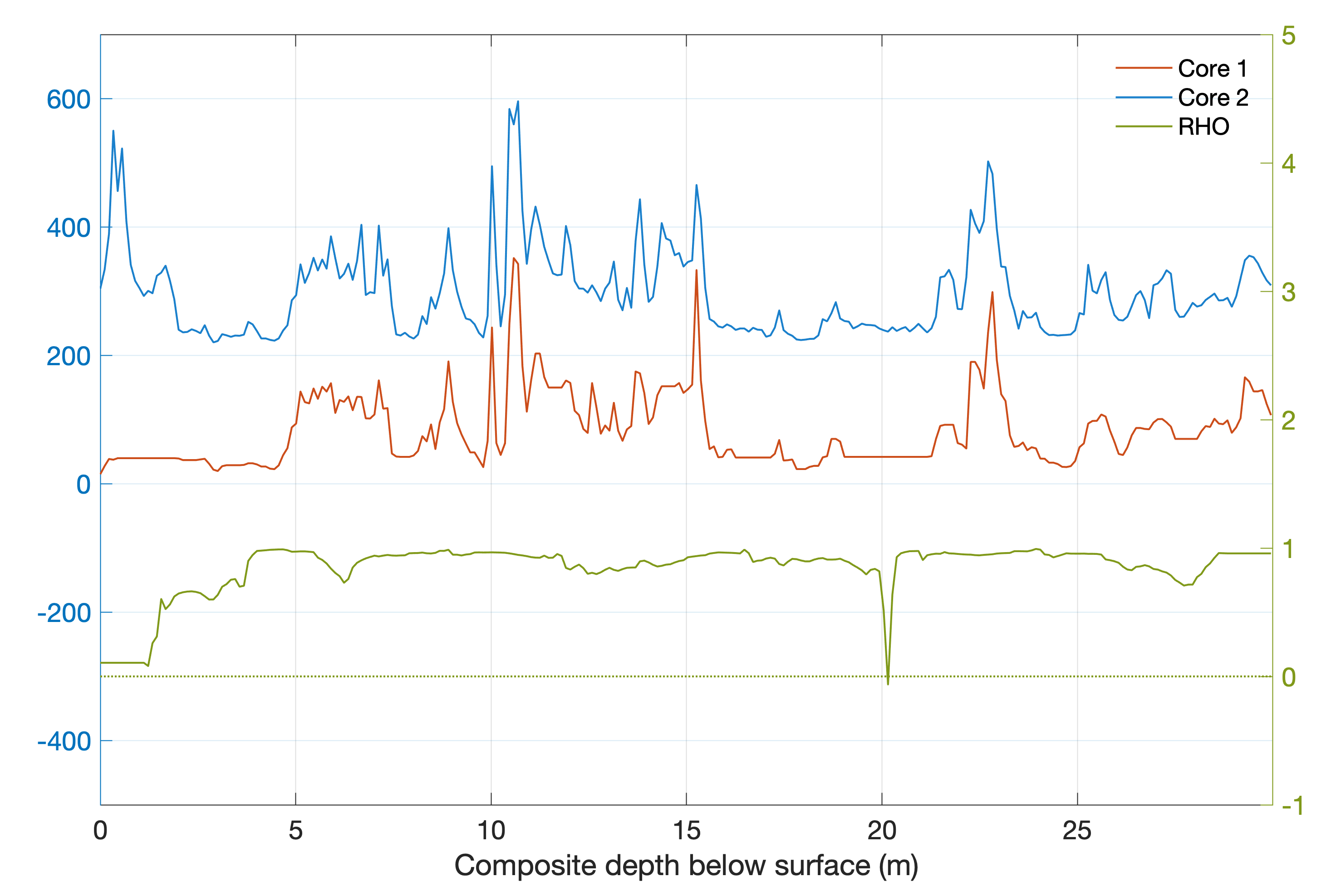
Display the aligned data with cross correlation by typing

figure('Position',[50 150 800 500])
axes('Box','On',...
    'XGrid','On',...
    'YGrid','On',...
    'YLim',[-500 700]), hold on
yyaxis left
line(data1i_int(:,1),data1i_int(:,2),...
    'Color',[0.8 0.3 0.1])
line(data2i_int(:,1),data2i_int(:,2)+200,...
    'Color',[0.1 0.5 0.8])
yyaxis right
line(data1i_int(:,1),corrt,...
    'Color',[0.5 0.6 0.1])
line(data1i_int(:,1),...
    zeros(size(data1i_int(:,1))),...
    'Color',[0.5 0.6 0.1],...
    'LineStyle',':')
set(gca,'YColor',[0.5 0.6 0.1],...
    'XLim',[0 max(data1(:,1))],...
    'YLim',[-1 5])
xlabel('Composite depth below surface (m)')
legend('Core 1','Core 2','RHO')
legend('boxoff')

References

Sakoe, Hiroaki, and Seibi Chiba. “Dynamic Programming Algorithm Optimization for Spoken Word Recognition.” IEEE® Transactions on Acoustics, Speech, and Signal Processing. Vol. ASSP-26, No. 1, 1978, pp. 43–49.
Paliwal, K. K., Anant Agarwal, and Sarvajit S. Sinha. “A Modification over Sakoe and Chiba’s Dynamic Time Warping Algorithm for Isolated Word Recognition.” Signal Processing. Vol. 4, 1982, pp. 329–333.