In geological drilling projects, two or more parallel cores often collected in order to compensate for core losses during drilling by overlapping sequences. Correlation of the core is a time-consuming and complex process that is usually done by very experienced geologists. In the Chew Bahir Drilling Project in Ethiopia, as part of the Hominin Sites and Paleolakes Drilling Projects (HSPDP), two parallel, almost 280 m long cores were collected in late 2014. The two cores are correlated using the Correlator software, which is part of the CoreWall package, but we also make experiments using manual and automated correlation using MATLAB. Here I present a script to perform a visual inspection and correlation of two cores using physical properties of the sediment such as the magnetic susceptibility.
The example is a hypothetical record of magnetic susceptibility from two 30 m long sediment cores. First, we have to define the segment of the core to be correlated, defined by the mimimum and maximum x-value, XMin and XMax, which could be depth below surface in meters. Second, we decide on the number of tiepoints n we wish to use to correlate the cores. Finally, we define the length w of the sliding window for which we calculate the cross-correlation of the cores after the adjustment of their depths.
XMin = 0;
XMax = 30;
n = 10;
w = 100;
Then import the sample data from files data_1.txt and data_2.txt.
data1 = load('data_1.txt');
data2 = load('data_2.txt');
We can then eliminate duplicate data points by typing
for i = 1:size(data1)-1
   if data1(i,1) == data1(i+1,1)
      data1(i,1) = NaN;
   end
end
data1(isnan(data1(:,1))==1,:) = [];
for i = 1:size(data2)-1
   if data2(i,1) == data2(i+1,1)
      data2(i,1) = NaN;
   end
end
data2(isnan(data2(:,1))==1,:) = [];
Define segment to be correlated:
data1 = data1(data1(:,1)>XMin & data1(:,1)<XMax,:);
data2 = data2(data2(:,1)>XMin & data2(:,1)<XMax,:);
Display the data using:
figure('Position',[150 300 1500 1100],...
    'Color','w');
% Axes 1
axes('Position',[0.1 0.85 0.8 0.12],...
    'Box','On',...
    'XLim',[XMin XMax],...
    'Color',[0.8 0.8 0.95],...
    'XGrid','On');
title('Core 1');
line(data1(:,1),data1(:,2),...
    'Marker','.',...
    'MarkerSize',3,...
    'Color',[0.1 0.3 0.8])
% Axes 2
axes('Position',[0.1 0.70 0.8 0.12],...
    'Box','On',...
    'XLim',[XMin XMax],...
    'Color',[0.8 0.8 0.95],...
    'XGrid','On');
title('Core 2');
line(data2(:,1),data2(:,2),...
    'Marker','.',...
    'MarkerSize',3,...
    'Color',[0.1 0.3 0.8])
% Axes 3
axes('Position',[0.1 0.40 0.8 0.12],...
    'Box','On',...
    'XLim',[XMin XMax],...
    'Color',[0.95 0.8 0.8],...
    'XGrid','On');
title('Define tiepoints in core 1 and 2!',...
    'Color','r',...
    'FontSize',24);
axis off
Pick a single pair of tie points in each of the two graphics and tune core 1 upon core 2 by interpolating the data.
for i = 1 : n
tiepoints1(i,:) = ginput(1);
tiepoints2(i,:) = ginput(1);
tietext = ['Tie Point ',num2str(i),' completed.'];
disp(tietext)
tielabels(i,:) = sprintf('%02.0f',i);
end
tune(1,:) = [0 0];
tune(2:size(tiepoints1,1)+1,1) = tiepoints1(:,1);
tune(2:size(tiepoints1,1)+1,2) = tiepoints2(:,1);
tune = sortrows(tune);
data1t(:,1) = interp1(tune(:,1),tune(:,2),...
    data1(:,1),'linear','extrap');
data1t(:,2) = data1(:,2);
close all
Interpolate the data after defining the tiepoints:
data1ti(:,1) = data2(:,1);
data1ti(:,2) = interp1(data1t(:,1),data1t(:,2), ...
      data1ti(:,1),'linear','extrap');
Calculate piecewise correlation
corrt(1,:) = length(data1ti)-w/2;
hwait = waitbar(0,'Please wait ...');
for i = w/2+1:length(data1ti)-w/2
[p,h] = corr(data1ti(i-w/2:i+w/2,2), ...
    data2(i-w/2:i+w/2,2));
corrt(1,i) = p;
waitbar(i/(length(data1ti)-w/2))
end
delete(hwait)
corrt(1,1:w/2) = corrt(1,w/2+1) * ones(1,w/2);
corrt(1,length(data1ti)-w/2+1:length(data1ti)) = ...
corrt(1,length(data1ti)-w/2) * ones(1,w/2);
corrt = corrt';
Display the results by typing
figure('Position',[150 300 1500 1100],...
'Color','w');
% Axes 1
axes('Position',[0.1 0.85 0.8 0.12],...
'Box','On',...
'XLim',[XMin XMax],...
'Color',[0.8 0.8 0.95],...
'XGrid','On');
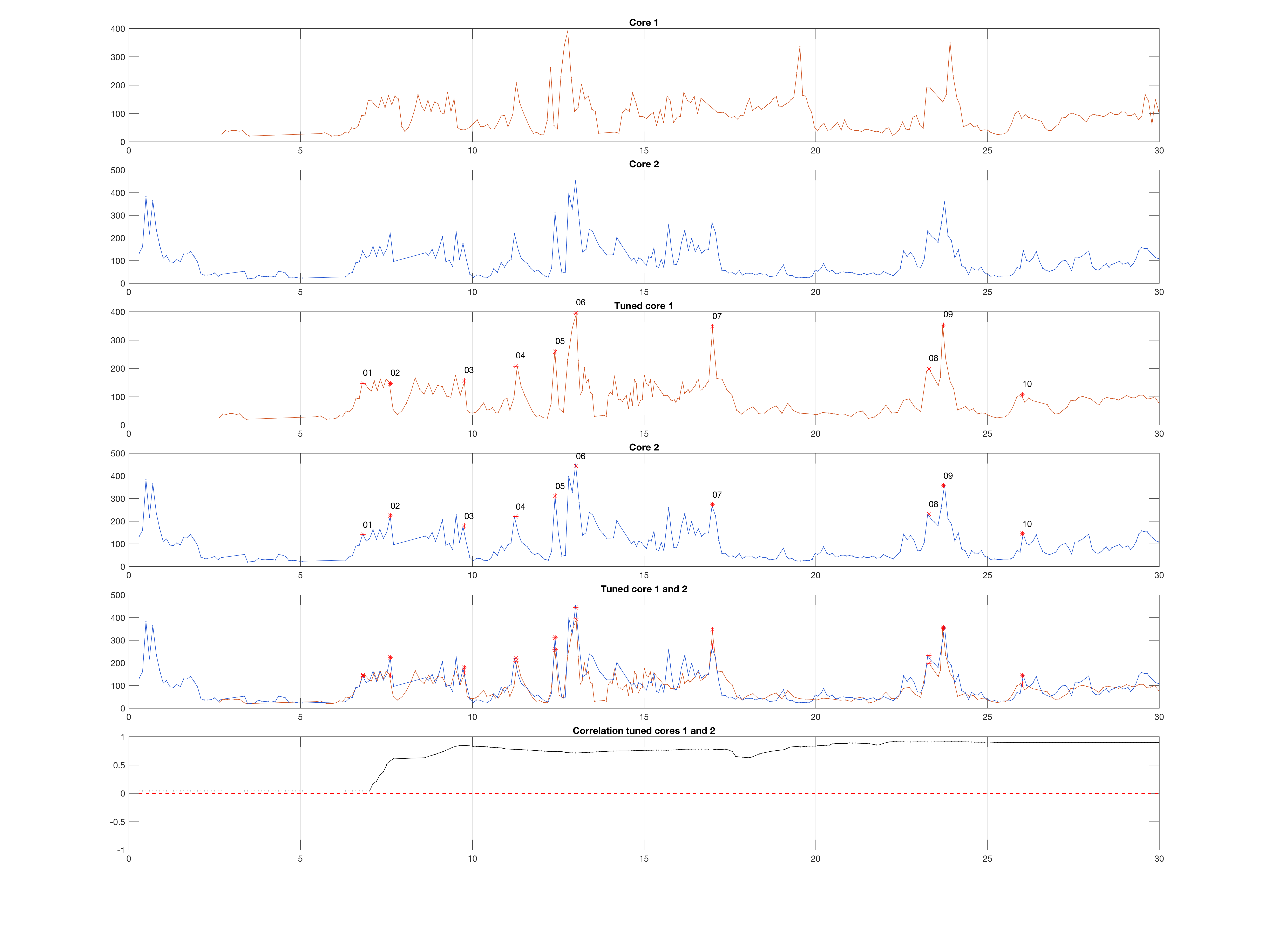
title('Core 1');
line(data1(:,1),data1(:,2),...
'Marker','.',...
'MarkerSize',3,...
'Color',[0.8 0.3 0.1])
% Axes 2
axes('Position',[0.1 0.70 0.8 0.12],...
'Box','On',...
'XLim',[XMin XMax],...
'Color',[0.8 0.8 0.95],...
'XGrid','On');
title('Core 2');
line(data2(:,1),data2(:,2),...
'Marker','.',...
'MarkerSize',3,...
'Color',[0.1 0.3 0.8])
% Axes 3
axes('Position',[0.1 0.55 0.8 0.12],...
'Box','On',...
'XLim',[XMin XMax],...
'Color',[0.95 0.8 0.8],...
'XGrid','On');
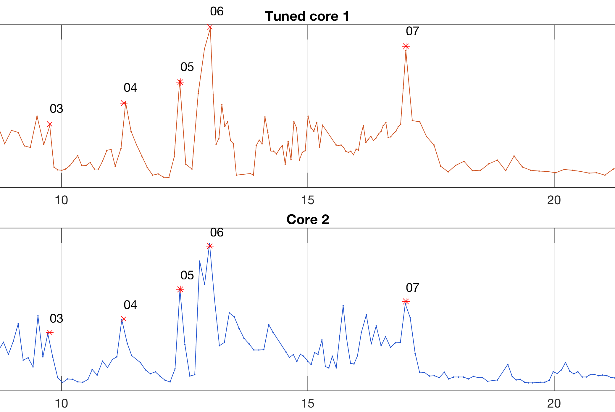
title('Tuned core 1');
line(data1t(:,1),data1t(:,2),...
'Marker','.',...
'MarkerSize',3,...
'Color',[0.8 0.3 0.1]), hold on
line(tiepoints2(:,1),tiepoints1(:,2),...
'LineStyle','None',...
'Marker','*',...
'Color','r')
text(tiepoints2(:,1),tiepoints1(:,2)+ ...
0.1*max(tiepoints1(:,2)),tielabels)
% Axes 4
axes('Position',[0.1 0.40 0.8 0.12],...
'Box','On',...
'XLim',[XMin XMax],...
'Color',[0.95 0.8 0.8],...
'XGrid','On');
title('Core 2');
line(data2(:,1),data2(:,2),...
'Marker','.',...
'MarkerSize',3,...
'Color',[0.1 0.3 0.8]), hold on
line(tiepoints2(:,1),tiepoints2(:,2),...
'LineStyle','None',...
'Marker','*',...
'Color','r')
text(tiepoints2(:,1),tiepoints2(:,2)+ ...
0.1*max(tiepoints2(:,2)),tielabels)
% Axes 5
axes('Position',[0.1 0.25 0.8 0.12],...
'Box','On',...
'XLim',[XMin XMax],...
'Color',[0.8 0.95 0.8],...
'XGrid','On');
title('Tuned core 1 and 2');
line(data1t(:,1),data1t(:,2),...
'Marker','.',...
'MarkerSize',3,...
'Color',[0.8 0.3 0.1]), hold on
line(tiepoints2(:,1),tiepoints1(:,2),...
'LineStyle','None',...
'Marker','*',...
'Color','r')
line(data2(:,1),data2(:,2),...
'Marker','.',...
'MarkerSize',3,...
'Color',[0.1 0.3 0.8]), hold on
line(tiepoints2(:,1),tiepoints2(:,2),...
'LineStyle','None',...
'Marker','*',...
'Color','r')
% Axes 6
axes('Position',[0.1 0.10 0.8 0.12],...
'Box','On',...
'XLim',[XMin XMax],...
'YLim',[-1 1],...
'Color',[0.8 0.95 0.8],...
'XGrid','On');
title('Correlation tuned cores 1 and 2');
line(data2(:,1),corrt(:,1),...
'Marker','.',...
'MarkerSize',3,...
'Color',[0 0 0]), hold on
line(data2(:,1),zeros(length(data2(:,1)),1),...
'Color',[1 0 0],...
'LineWidth',1,...
'LineStyle','--')
clear axes* figure* title* i n
This results in a figure window with six graphics (click to enlarge):
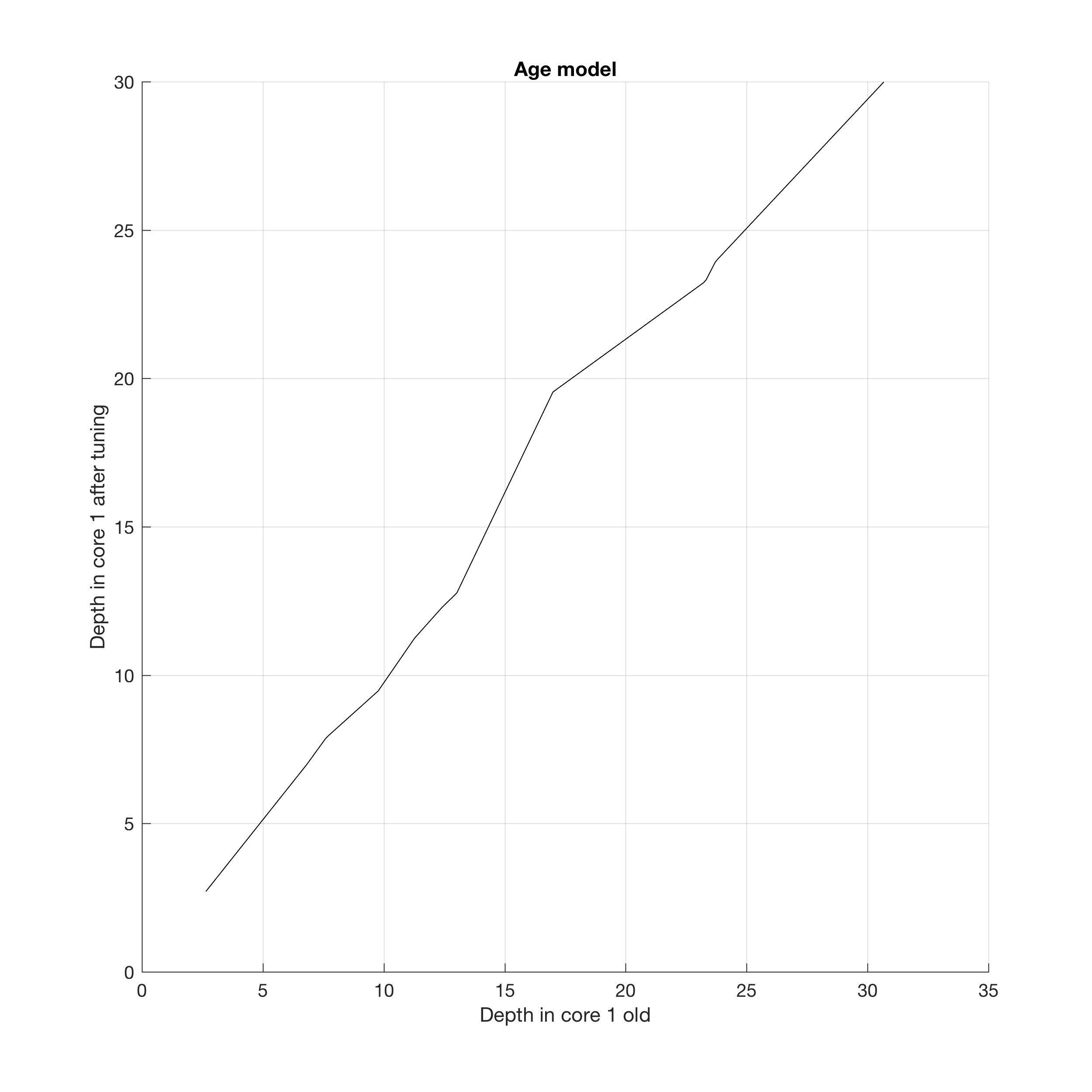
You can display the age model by typing
figure('Position',[2000 200 600 600],...
    'Color','w');
axes('XGrid','On',...
    'YGrid','On');
title('Age model');
xlabel('Depth in core 1 old')
ylabel('Depth in core 1 after tuning')
line(data1t(:,1),data1(:,1),...
    'Color',[0 0 0])