
Anyone who has ever dealt with the statistical analysis of compositional data must have stumbled across John Aitchison’s (1926-2016) log-ratio transformation. The Scottish statistician spent much of his career on the statistics of such data, wrote the famous book “The Statistical Analysis of Compositional Data” (Aitchison, 1986, 2003) and multiple papers on the same topic, with associated MATLAB 5 software package CODA available from the author at the time of publication, updated versions now available for download at CoDAWeb. Aitchison’s log-ratio transformation overcomes the close-sum problem of closed data, i.e. data expressed as proportions and adding up to a fixed total such as 100 percent. The close-sum problem causes spurious negative correlations between pairs of variables that are avoided by logarithmizing ratios of the variables. Here is a simple MATLAB example illustrating the effect of Aitchison’s log-ratio transformation on compositional data.
We are currently evaluating our data from the cores of the Chew Bahir project. These are often closed data, i.e. they are very much influenced by dilution effects. In the simplest example, this could be a mixture of three components, which together make up 100% of the sediment. Imagine that one of the components is now constant, i.e. the same amount of this component is always delivered per time. Since all three components are always 100%, the other two components are necessarily anticorrelated: one goes up and other one goes down by the same amount.
Using ratios helps to overcome the problem that the magnitudes of compositional data are actually ratios whose denominators are the sum of all constituents (see Davis, 2003, for a short summary of Aitchison’s log-ratio transformation). Product-moment covariances of ratios, however, are awkward to manipulate, cause complicated products and quotients. John Aitchison therefore suggested to take the logarithms of those ratios, taking advantage of the simple properties of the logarithmic function, such as log(x/y) = log(x)-log(y), and hence log(x/y) = -log(y/x), which allows a significant reduction in the number of covariances necessary to describe the data set (Aitchison, 2003, p. 65-66).
Here is a simple MATLAB example illustrating the closed-sum problem of a system with three variables, and the use of ratios as well as log-ratios to overcome the problem of spurious correlations between pairs of variables. First, we clear the workspace and choose colors for the plots.
clear, close all, clc
colors = [
0 114 189
217 83 25
237 177 32
126 47 142
]./255;
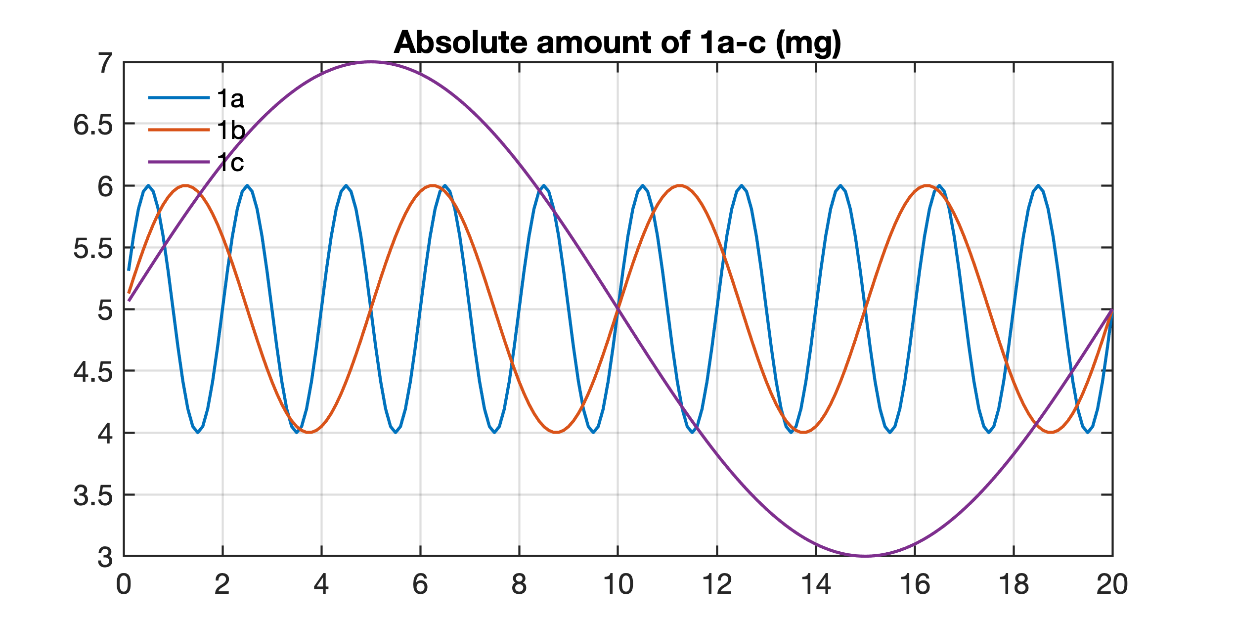
We are interested in element 1a and element 1b, which are diluted by element 1c. We simply create three variables with magnitudes measured in milligrams, contributing to a sediment and with a sinusoidal variation of 200 samples down core. Make sure that all absolute values are >0.
t = 0.1 : 0.1 : 20; t = t';
element1a = sin(2*pi*t/2) + 5;
element1b = sin(2*pi*t/5) + 5;
element1c = 2*sin(2*pi*t/20) + 5;

figure('Position',[100 1000 600 300])
a1 = axes('Position',[0.1 0.1 0.8 0.8],...
  'Box','On',...
  'LineWidth',1,...
  'FontSize',14);
line(a1,t,element1a,...
  'Color',colors(1,:),...
  'LineWidth',1.5);
line(a1,t,element1b,...
  'Color',colors(2,:),...
  'LineWidth',1.5);
line(a1,t,element1c,...
  'Color',colors(4,:),...
  'LineWidth',1.5);
legend('1a','1b','1c',...
  'Box','Off',...
  'Location','northwest'), grid
title('Absolute amount of 1a-c (mg)')
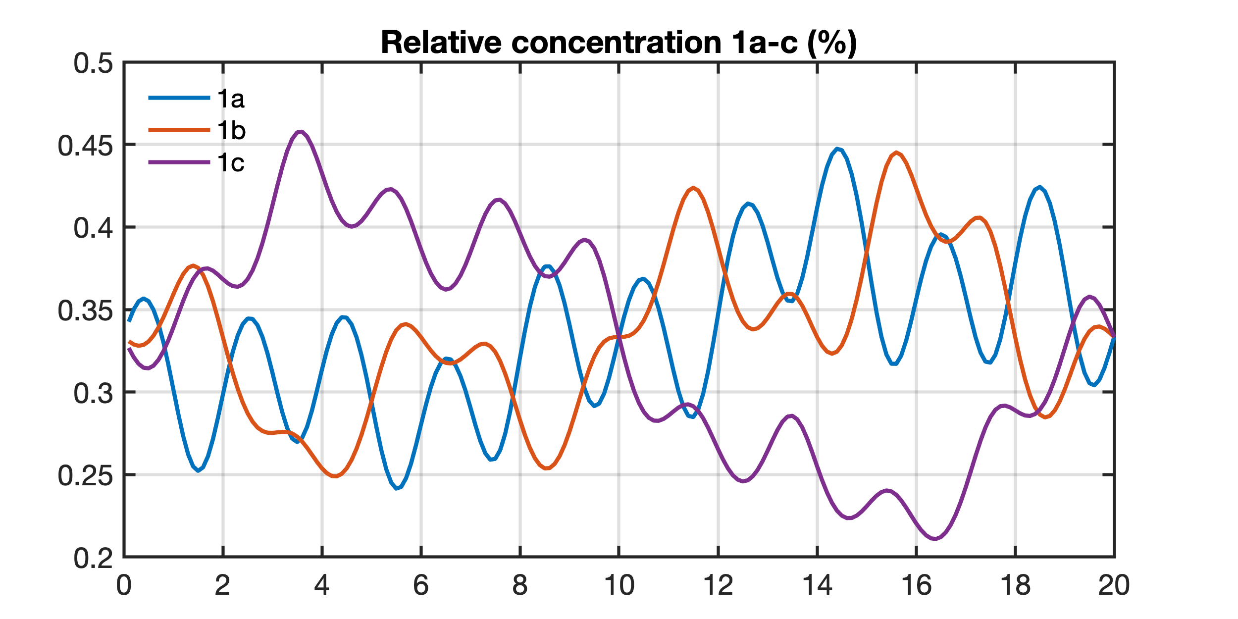
Calculating percentages of elements 1a-c, i.e. creating ratios of the individual elements and the sum of all elements. This process creates closed data, i.e. the data are now expressed as proportions and adding up to a fixed total of 100 percent, 1a+1b+1c = 100%. Now elements 1a and elements 1b are affected by the dilution by elements 1c. These elements show a significant sinusoidal long-term trend that is not real, as the first figure shows.
element1a_perc = element1a./...
  (element1a+element1b+element1c);
element1b_perc = element1b./...
  (element1a+element1b+element1c);
element1c_perc = element1c./...
  (element1a+element1b+element1c);

figure('Position',[100 700 600 300])
a2 = axes('Position',[0.1 0.1 0.8 0.8],...
  'Box','On',...
  'LineWidth',1.5,...
  'FontSize',14);
line(a2,t,element1a_perc,...
  'Color',colors(1,:),...
  'LineWidth',1.5);
line(a2,t,element1b_perc,...
  'Color',colors(2,:),...
  'LineWidth',1.5);
line(a2,t,element1c_perc,...
  'Color',colors(4,:),...
  'LineWidth',1.5);
legend('1a','1b','1c',...
  'Box','Off',...
  'Location','northwest'), grid
title('Relative concentration 1a-c (%)')
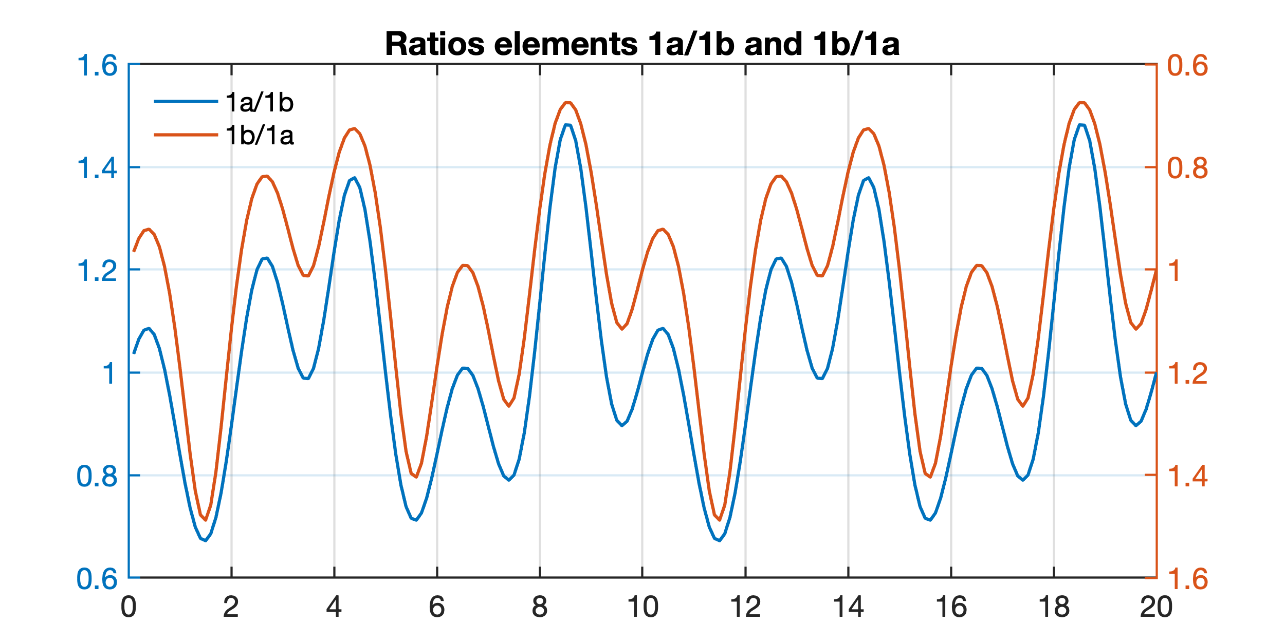
Built ratios of element 1a/1b and element 1b/1a, which are both independent from element 1c. Note the change of sign and difference in the amplitudes. The ratio of element 1a/1b and 1b/1a do not show the trend caused by the dilution effect of element 1c. However, the two curves are not identical, i.e. 1a/1b and 1b/1a are not symmetric (see Weltje and Tjallingii 2008, page 426).
ratio12 = element1a_perc./element1b_perc;
ratio21 = element1b_perc./element1a_perc;

figure('Position',[100 400 600 300])
a3 = axes('Position',[0.1 0.1 0.8 0.8],...
  'Box','On',...
  'LineWidth',1,...
  'FontSize',14);
yyaxis left, line(a3,t,ratio12,...
  'Color',colors(1,:),...
  'LineWidth',1.5);
yyaxis right, line(a3,t,ratio21,...
  'Color',colors(2,:),...
  'LineWidth',1.5);
set(a3,'YDir','Reverse')
legend('1a/1b',...
  '1b/1a',...
  'Box','Off',...
  'Location','northwest'), grid
title('Ratios elements 1a/1b and 1b/1a')
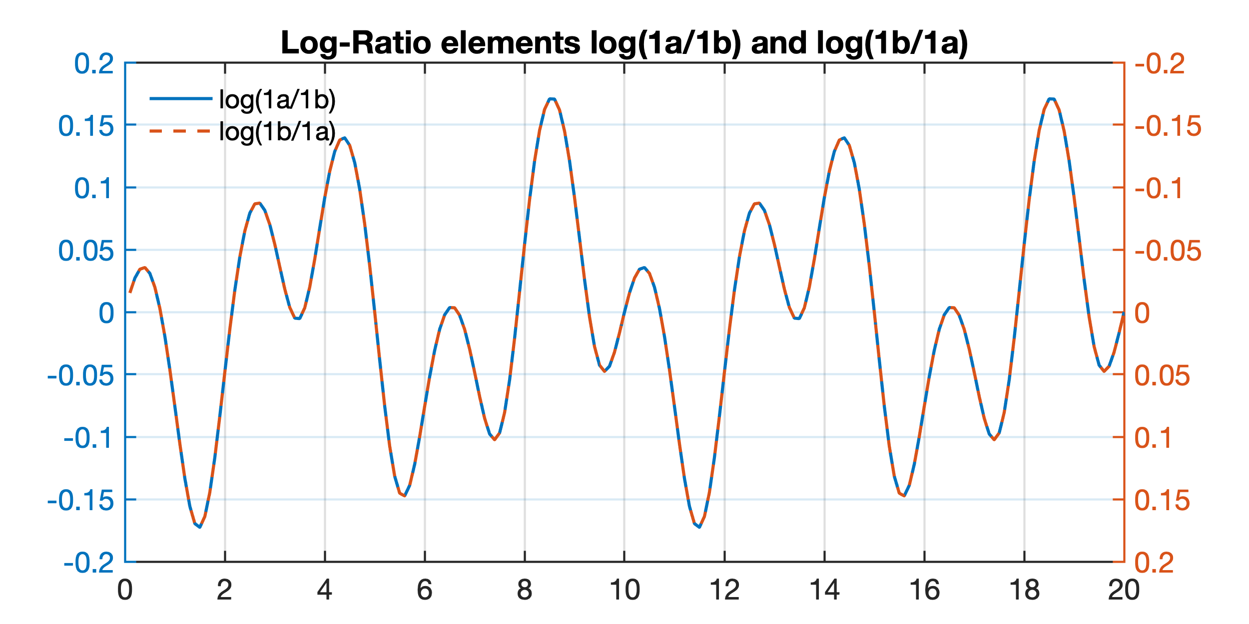
Display log-ratios instead according to Aitchison (1986, 2003). The log- ratios log(1a/1b) and log(1b/1a) are identical except for the sign. Hence it makes no difference whether we use log(1a/1b) or log(1b/1a), for instance, when running further statistical analysis on the data.
ratio12log = log10(ratio12);
ratio21log = log10(ratio21);

figure('Position',[100 100 600 300])
a4 = axes('Position',[0.1 0.1 0.8 0.8],...
  'Box','On',...
  'LineWidth',1,...
  'FontSize',14);
yyaxis left
line(a4,t,ratio12log,...
  'Color',colors(1,:),...
  'LineWidth',1.5);
yyaxis right
line(a4,t,ratio21log,...
  'Color',colors(2,:),...
  'LineStyle','--',...
  'LineWidth',1.5);
set(a4,'YDir','Reverse')
legend('log(1a/1b)',...
  'log(1b/1a)',...
  'Box','Off',...
  'Location','northwest'), grid
title('Log-Ratio elements log(1a/1b) and log(1b/1a)')
Comments are, as always, very welcome via email to me!
References:
Aitchison, J., 1986, 2003, The Statistical Analysis of Compositional Data. Blackburn PR, 460 pages.
Aitchison, J., 1999, Logratios and natural laws in compositional data analysis, Mathematical Geology, 31, 563-580.
Croudace, I.W., Rothwell, R.G. , 2015, Twenty Years of XRF Core Scanning Marine Sediments: What Do Geochemical Proxies Tell Us? in: Croudace, I.W., Rothwell, R.G. (eds.), 2015, Micro-XRF Studies of Sediment Cores, Springer. -> See page 50, “Plotting Core Scanner Data, the Importance of Normalisation and Log-Ratios”.
Davies, S.J., Lamb, H.F., Roberts, S.J., 2015, Micro-XRF Core Scanning in Palaeolimnology: Recent Developments, in: Croudace, I.W., Rothwell, R.G. (eds.), 2015, Micro-XRF Studies of Sediment Cores, Springer, Heidelberg.
Davis, J.C., 2002, Statistics and Data Analysis in Geology, Third Edition, John Wiley & Sons, New York.
Martín-Ferández, J.A., Thió-Henestrosa, S. (Eds.), 2016, Compositional Data Analysis, CoDaWork, L’Escala, Spain, June 2015, Springer Proceedings in Mathematics & Statistic, Volume 187, Springer.
van den Boogaart, K.G., Tolosana-Delgado, R., 2013, Analyzing Compositional Data with R, Use R! Springer, Heidelberg.
Pearson, K., 1897, Mathematical contributions to the theory of evolution. On a form of spurious correlation which may arise when indices are used in the measurement of organs. Proceedings of the Royal Society of London, LX, 489-502.
Weltje, G.J., Tjallingii, R., 2008, Calibration of XRF core scanners for quantitative geochemical logging of sediment cores: Theory and application, Earth and Planetary Science Letters, 274, 423-438.