
During a workshop on time series analysis on paleoclimatic data, I was asked how data gaps affect the results of spectral analyzes. The good news is, the expected climatic cycles such as Milankovitch cycles do not shift when the time series has gaps. However, it is important that the data is properly pre-treated before being examined with a method of spectral analysis.
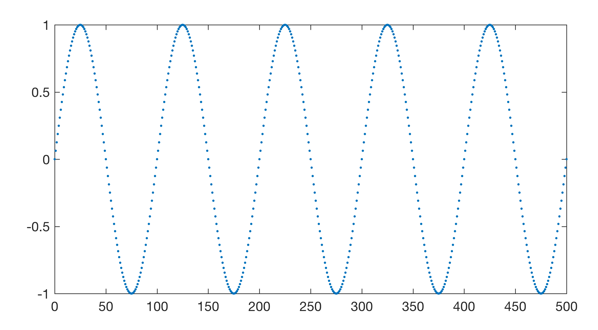
This examples creates a synthic periodic signal, introduces gaps and then calculates the Fast Fourier Transform (FFT) based power spectrum of an interpolated evenly-spaced version of the signal and the Lomb-Scargle (LS) based power spectrum of the unevenly-spaced version of the signal without interpolation. The recipes for both methods are taken from Chapter 5 of the MRES book. First we create a synthetic data set, which is a sine wave with a period of 100.
clear, clc
data(:,1) = 0 : 500;
data(:,2) = sin(2*pi*data(:,1)/100);
figure('Position',[200 600 600 300])
axes('Box','On',...
   'LineWidth',0.6,...
   'FontSize',12)
line(data(:,1),data(:,2),...
   'Color',[0 0.4453 0.7383],...
   'LineStyle','None',...
   'Marker','.')
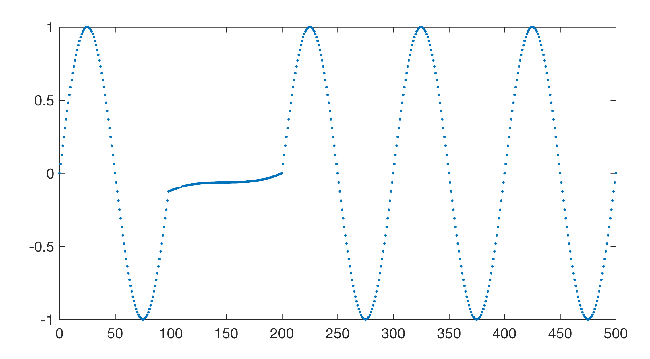
Then we introduce gaps by removing the 100th to 200th data point in data.
datag = data;
datag(100:200,:) = [];
figure('Position',[200 600 600 300])
axes('Box','On',...
   'LineWidth',0.6,...
   'FontSize',12)
line(datag(:,1),datag(:,2),...
   'Color',[0 0.4453 0.7383],...
   'LineStyle','None',...
   'Marker','.')

FFT-based spectral analysis methods require evenly-spaced data without gaps. Numerous methods exist for interpolating unevenly-spaced sequences of data or time series. The aim of these interpolation techniques for x(t) data is to estimate the x-values for an equally-spaced t vector from the irregularly-spaced x(t) actual measurements. Linear interpolation predicts the x-values by effectively drawing a straight line between two neighboring measurements and by calculating the x-value at the appropriate point along that line. However, this method has its limitations. It assumes linear transitions in the data, which introduces a number of artifacts including the loss of high-frequency components of the signal and the limiting of the data range to that of the original measurements.
Cubic-spline interpolation is another method for interpolating data that are unevenly spaced. Cubic splines are piecewise continuous curves requiring at least four data points for each step. The method has the advantage that it preserves the high-frequency information contained in the data. However, steep gradients in the data sequence, which typically occur adjacent to extreme minima and maxima, could cause spurious amplitudes in the interpolated time series. The function pchip provides an alternative to linear and classic spline interpolation. The name pchip stands for Piecewise Cubic Hermite Interpolating Polynomial and this method performs a shape-preserving piecewise cubic interpolation. The function avoids the typical artifacts of the splines as it preserves the original shape of the data series.
datai(:,1) = 0 : 500;
datai(:,2) = pchip(datag(:,1), ...
   datag(:,2),datai(:,1));

figure('Position',[200 600 600 300])
axes('Box','On',...
   'LineWidth',0.6,...
   'FontSize',12)
line(datai(:,1),datai(:,2),...
   'Color',[0 0.4453 0.7383],...
   'LineStyle','None',...
   'Marker','.')
Since all these (and other) interpolation techniques might introduce artifacts into the data, it is always advisable to (1) keep the total number of data points constant before and after interpolation, (2) report the method employed for estimating the evenly-spaced data sequence, and (3) explore the effect of interpolation on the variance of the data. We then calculate FFT-based power spectrum of original data series, of the series with gaps and the interpolated series.
clf
[Pxx,f] = periodogram(data(:,2),[],512,1);
[Pixx,f] = periodogram(datai(:,2),[],512,1);

figure('Position',[200 600 600 300])
axes('Box','On',...
   'LineWidth',0.6,...
   'FontSize',12)
line(f,abs(Pxx),...
   'LineWidth',1,...
   'Color',[0 0.4453 0.7383])
axis([0 0.03 0 250]), grid, hold on
line(f,abs(Pixx),...
   'Color',[0.8477 0.3242 0.0977],...
   'LineWidth',1)
axis([0 0.03 0 250]), grid
legend('Original','Interpolated')
legend boxoff
xlabel('Frequency')
ylabel('Power')
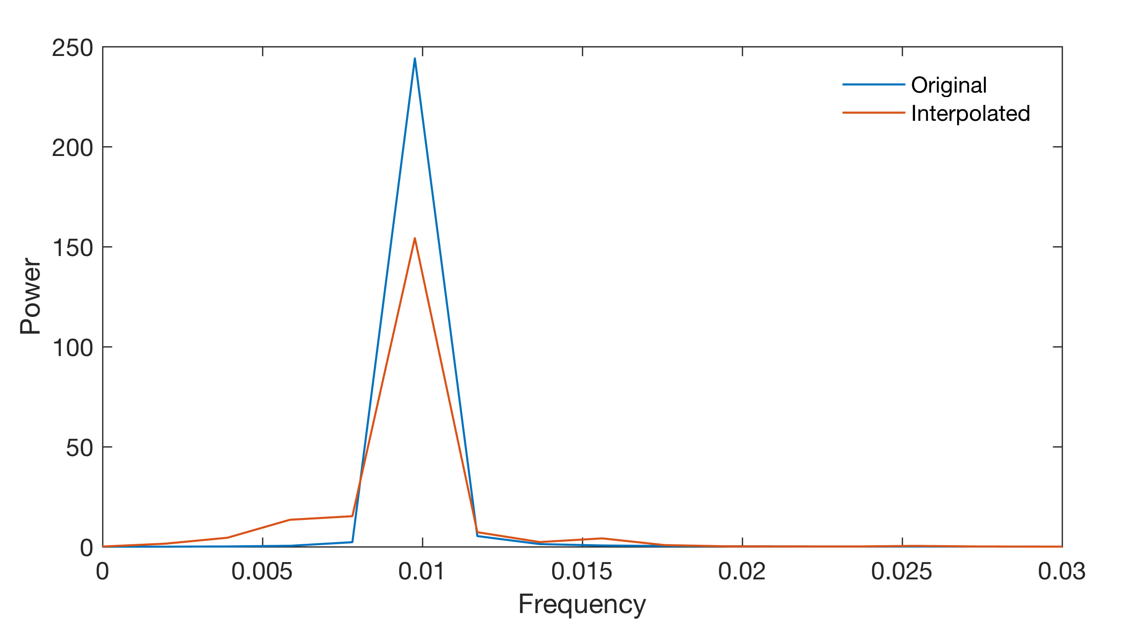
As we can see, the height of the spectral peak is slightly lower than the data without gaps. Although interpolating the unevenly-spaced data to a grid of evenly- spaced times is one way to overcome this problem, interpolation introduces numerous artifacts into the data, in both the time and frequency domains. For this reason an alternative method of time-series analysis has become increasingly popular in earth sciences, the Lomb-Scargle algorithm (e.g., Scargle 1981, 1982, 1989, 1990, Press et al. 1992, Schulz et al. 1998). Calculate LS spectrum of original data and the one with gaps using the code from the MRES book.
clf, clear f p*
t = data(:,1);
x = data(:,2);

int = mean(diff(t));
ofac = 4; hifac = 1;
f = ((2*int)^(-1))/(length(x)*ofac): ...
    ((2*int)^(-1))/(length(x)*ofac): ...
    hifac*(2*int)^(-1);

x = x - mean(x);

for k = 1:length(f)
    wrun = 2*pi*f(k);
    px(k) = 1/(2*var(x)) * ...
    ((sum(x.*cos(wrun*t - ...
    atan2(sum(sin(2*wrun*t)), ...
    sum(cos(2*wrun*t)))/2))).^2) ...
    /(sum((cos(wrun*t - ...
    atan2(sum(sin(2*wrun*t)), ...
    sum(cos(2*wrun*t)))/2)).^2)) + ...
    ((sum(x.*sin(wrun*t - ...
    atan2(sum(sin(2*wrun*t)), ...
    sum(cos(2*wrun*t)))/2))).^2) ...
    /(sum((sin(wrun*t - ...
    atan2(sum(sin(2*wrun*t)), ...
    sum(cos(2*wrun*t)))/2)).^2));
end

t = datag(:,1);
x = datag(:,2);

int = mean(diff(t));
ofac = 4; hifac = 1;
fg = ((2*int)^(-1))/(length(x)*ofac): ...
    ((2*int)^(-1))/(length(x)*ofac): ...
    hifac*(2*int)^(-1);

x = x - mean(x);

for k = 1:length(fg)
    wrun = 2*pi*fg(k);
    pxg(k) = 1/(2*var(x)) * ...
    ((sum(x.*cos(wrun*t - ...
    atan2(sum(sin(2*wrun*t)), ...
    sum(cos(2*wrun*t)))/2))).^2) ...
    /(sum((cos(wrun*t - ...
    atan2(sum(sin(2*wrun*t)), ...
    sum(cos(2*wrun*t)))/2)).^2)) + ...
    ((sum(x.*sin(wrun*t - ...
    atan2(sum(sin(2*wrun*t)), ...
    sum(cos(2*wrun*t)))/2))).^2) ...
    /(sum((sin(wrun*t - ...
    atan2(sum(sin(2*wrun*t)), ...
    sum(cos(2*wrun*t)))/2)).^2));
end
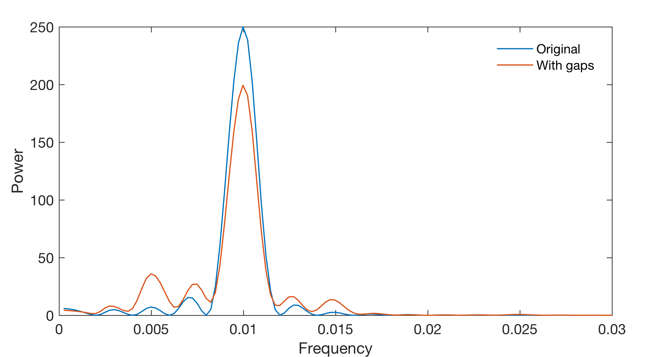
We display the results of the LS analysis of the data without gaps and the data with gaps for comparison.
figure('Position',[200 600 600 300])
axes('Box','On',...
   'LineWidth',0.6,...
   'FontSize',12)
line(f,px,'LineWidth',1,...
   'Color',[0 0.4453 0.7383])
axis([0 0.03 0 250]), grid, hold on
line(fg,pxg,...
   'Color',[0.8477 0.3242 0.0977],...
   'LineWidth',1)
axis([0 0.03 0 250]), grid
legend('Original','With gaps')
legend boxoff
xlabel('Frequency')
ylabel('Power')
Also in this example, using the LG algorithm, gaps do not shift the spectral peaks but reduce the actual amplitude.
References
Lomb NR (1972) Least-Squared Frequency Analysis of Unequally Spaced Data. Astrophysics and Space Sciences 39:447–462
Press WH, Teukolsky SA, Vetterling WT (2007) Numerical Recipes: The Art of Scientific Computing – Third Edition. Cambridge University Press, Cambridge
Scargle JD (1981) Studies in Astronomical Time Series Analysis. I. Modeling Random Processes in the Time Domain. The Astrophysical Journal Supplement Series 45:1–71
Scargle JD (1982) Studies in Astronomical Time Series Analysis. II. Statistical Aspects of Spectral Analysis of Unevenly Spaced Data. The Astrophysical Journal 263:835–853
Scargle JD (1989) Studies in Astronomical Time Series Analysis. III. Fourier Transforms, Autocorrelation Functions, and Cross-Correlation Functions of Unevenly Spaced Data. The Astrophysical Journal 343:874–887
Schulz M, Stattegger K (1998) SPECTRUM: Spectral Analysis of Unevenly Spaced Paleoclimatic Time Series. Computers & Geosciences 23:929–945