
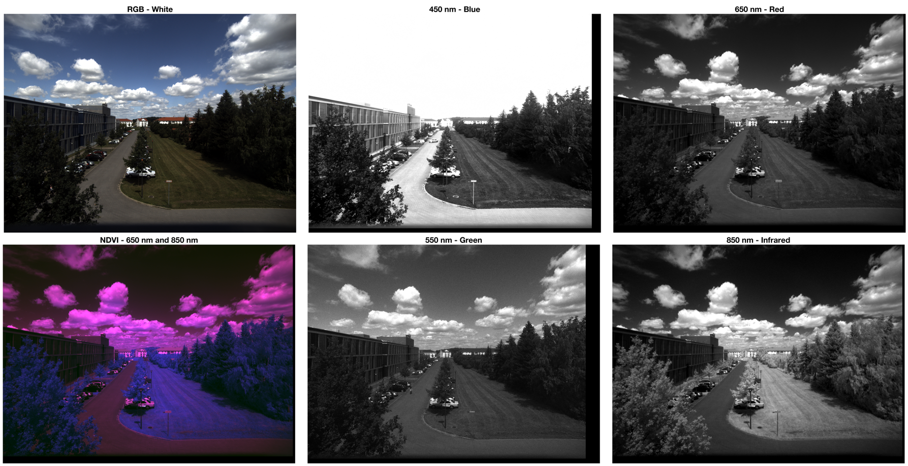
Using the MAPIR Survey2 cameras described in an earlier post I took photos of the car park next to our departmental building. The relatively inexpensive multispectral array consists of four cameras, ~340 € each, recording NDVI Red+NIR (650 and 850 nm), Blue (450 nm), Green (550 nm) and Visible Light RGB (~370–650 nm). We use the four cameras to build a multispectral array, possibly mounted on drones, to determine various types of minerals, vegetation, and man-made materials on the ground.
I load the four raw images using the script described in the NDVI exercise and adjust the image intensity values using the function imadjust and use the script described in Chapter 8.5 of MRES to register the image.
The intensity images of the spectral bands nicely demonstrate the strength of multispectral imaging in determining types of materials on the ground. When doing this, spectral libraries such as the USGS Spectral Library, are used to identify the various materials based on their characteristic absorption bands. In some applications, absorption intensity ratios are used to create images to distinguish the materials in the image.
As an example, the NDVI is an index to map live green vegetation. The index is based on the ratio of the difference of the red and infrared radiances. The pigments of plants strongly absorb visible light (400–700 nm) for the use in photosynthesis, whereas it reflects near-infrared light (700–1100 nm). In our example, the trees in the picture are dark gray in the Red (650 nm) spectral band, corresponding to low reflectance values, whereas the trees are light gray in the NIR (850 nm) spectral band.