In a series of blog posts, I will tell you a little about how I teach computational geosciences with MATLAB. On the first half of day 3 of the one-week course I teach time-series analysis.
Teaching time series analysis is a major challenge. One reason for this is the fact that basic knowledge of the Fourier analysis and Fourier transformation are unknown to many students. For these students changing from the time domain to the frequency domain is associated with great difficulties. If, however, the principle is understood, the advantage of the frequency domain in time series analysis, but also in signal processing, is quickly apparent.
To ensure easy access, we work consistently with synthetic data. Here, we add sinusoidal signals, a trend and normally distributed noise, in order to then separate the components again using time series analysis methods. I also use the sound of the signals with the MATLAB function sound, as described in the interactive version of MRES and in an earlier blog entry.
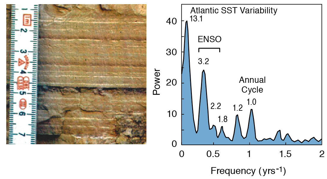
I start with FFT-based methods like the periodogram, deal with it very extensively before I use alternative methods like Lomb-Scargle or Wavelets. I have also recently experimented with nonlinear methods like recurrence plots, using the corresponding section of MRES written by my colleague Norbert Marwan.
The enthusiasm of the participants is usually great when the first periodogram appears on the screen, even if the mathematical principles are often not fully understood. If the Lomb-Scargle Periodogram or Wavelet Powerspectrum with the same synthetic data appears afterwards, the success of the course is almost certain!
The time series analysis is also part of the course on which most of the email requests are made in the weeks following the event. In this case, there are still minor or major problems with the application to the participant’s own data, which, however, can usually be solved by exchanging and discussing MATLAB scripts.