

Artificial neural networks (ANNs) are widely used in the geosciences. There are numerous convenient tools in MATLAB and the Deep Learning Toolbox that make it easy to get started, but the examples used in the documentation, tutorials and are usually very complex. Here is a very simple MATLAB example.
Introduction
I searched textbooks, technical articles and internet blogs for the simplest possible example of an ANN with backpropagation. Most of the examples are already so complicated that they do not offer a good introduction for someone who has no prior knowledge. On the other hand, an increasing number of people are using methods from the field of artificial intelligence and deep learning without first familiarizing themselves with the basics.
In the following I show a simple MATLAB script for an ANN, which is inspired by an example that can be found in several variants on the Internet. Since these blog posts do not follow scientific rules, sources are usually not cited. One of the oldest sources is a blog post by Andrew Trask (2015), where you can find the well-documented Python code of a simple network, but with an error in the activation function.
For an easy introduction to the topic of machine learning in general and ANN in particular, I would like to recommend the excellent videos on Grant Sanderson’s 3Bue1Brown YouTube channel, which have become very popular. On his website or on the YouTube Channel you will find a section about ANNs in general including the introduction “But what is a Neural Network?“. There is nothing comparable on the web that explains complex topics in maths and computer science with such simple, yet skilfully crafted animations.
Next, I would like to recommend the Online Training Courses from MathWorks, which contains some free short introductions, for example the Machine Learning Onramp and Deep Learning Onramp, which guides you through some theoretical concepts and a simple MATLAB example within approximately 2–2.5 hours. If you have access to the MATLAB Academy, for example through a MATLAB Site Licence / Total Academic Headcount Licence from your university, you can take advantage of many more self-paced online training courses on the topic, e.g. a 12-hour course on Machine Learning with MATLAB or a 7-hour course on Deep Learning with MATLAB.
An ANN with backpropagation attempts to predict the output from the inputs. The error is used to iteratively improve the weights of the ANN. The weights are the ANN, the improvement of the weights is the learning of the ANN. In our example, we use the inputs and outputs from the above example by Trask (2015), which can also be found in other Internet examples, as well as weights whose initial value is zero in each case.
Another source of inspiration for the following example was the articles on artificial neural networks and backpropagation on the German and English Wikipedia pages. Unfortunately, as is so often the case on Wikipedia, these pages are incomplete, do not always include references and are sometimes inaccurate or even partially incorrect. In the following example, however, the variable names and the step-by-step explanation are based on the German Wikipedia article (2024). There you will also find a number of useful graphics to explain ANNs.
I would also like to thank Dr Kathi Kugler (MathWorks) for her support and comments while working on this example.
Step 1 – Designing the Artificial Neural Network
We first clear the workspace using clear.
clear
Here we can define a learning rate or step size to improve the weights. As always with such algorithms, the rate is a compromise between fast learning and accurate learning. You can play around with different values for alp and see the difference in the graphics below.
alp = 0.1;
Input layer of the ANN – Our training data set consists of four samples of three values each, such as four different samples of climate transitions characterized by three parameters, such as mean, standard deviation and skewness. We create a very simple ANN with an input layer with three input nodes / three artificial neurons corresponding to the three parameters.
x = [0 0 1
     1 1 1
     1 0 1
     0 1 1];
Output layer of the ANN – This is the expected output of the training data set, e.g. the Type 1 or 2 of the respective climate transition of the four samples in the training data set. As you can see, the first and last sample should be characterized by Type 0 of climate transition and the second and third sample should be of Type 1. We have only one column and therefore only one output node.
y = [0
     1
     1
     0];
The weights – The ANN essentially consists of the matrix of weights w. In our example, we only have one set of three weights w because we only have one input layer x and one output layer y, which are linked by the weights w (see graphical representation of the network below). We choose weights w with an initial value of zero, but in other examples such as the one by Trask (2015) random numbers normalized to a total of one are used. In any case, the weights w are iteratively improved through backpropagation, i.e. we calculate an estimate of the output oj based on these weights w, calculate an error, e.g. the difference between expected output y and predicted output oj, which is then used, together with the learning rate / step size alp from above to update the weights w / replace them by an improved set of weights w. Improving the weights w is the learning of the ANN. We have three nodes, so we also have three weights.
w = [0
     0
     0];
We train the network in which the best values for the weights w are to be found in order to find oj as a prediction oj of the output y.
Step 2 – Training the Artificial Neural Network
for i = 1 : 10000
When the neuron receives the input x it first computes a propagation function netj, which usually is the sum of the input x weighted by w or, in other words, the inner product of x and w.
netj = x*w;
After the propagation function netj, the activation function is applied, which brings the nonlinearity into the network, to compute an estimate of the output oj. There are many different functions used as activation function. The ReLU function is often used in the hidden layers (not used here), while the sigmoid function sigfct (see below) is used in the output layer:
oj = sigfct(netj);
The extent to which the result oj from the neural network deviates from the target value y is determined with the help of an error function. There are different types of error functions, for example the mean squared error
E = mean((y - oj).^2);
if the neural network returns only one single value. In our example, we use the difference between calculated and expected outputs (oj – y), which provides the three values required to update the three weights w. We use, however, the mean squared error for the graphical display of the learning process (see below). The weights w can now be adjusted using the stepsize alph, the inputs x of the training data set, the gradients dw determined using backpropagation and the error (oj – y). This is not fully explained in the German Wikipedia article on artifical neural networks (2024), but in the German Wikipedia article on backpropagation (2024) it becomes clear if you don’t want to calculate the partial derivatives according to the chain rule yourself. I have omitted the minus sign in front of alp, as it is written in Wikipedia (2024b), instead dw is then subtracted from w in the next line, as written in Wikipedia. Alternatively, you can also turn (oj – y) around, as in the mean squared error E above. However, the two Wikipedia articles do not match at this point with regard to the sign of the correction of the weights w.
dw = alp*x'*(sigfctderiv(netj).*(oj - y));
In the second step, the gradients dw are used in an optimization procedure to obtain improved weights w with a lower error – this is how the network learns. The criterion for terminating the procedure can be the number of iterations or the error falls below a threshold value. This is the usual procedure, as already known from other adaptive procedures such as adaptive filters.
w = w - dw;
We store the values for the mean squared error E, the prediction of the output oj and the weights w for each i of the for loop in order to graphically represent the iterative learning of the network below.
   Ei(:,i) = E;
   oji(:,i) = oj;
   wi(:,i) = w;
End of the for loop.
end
Step 3 – Evaluating the ANN Training Results
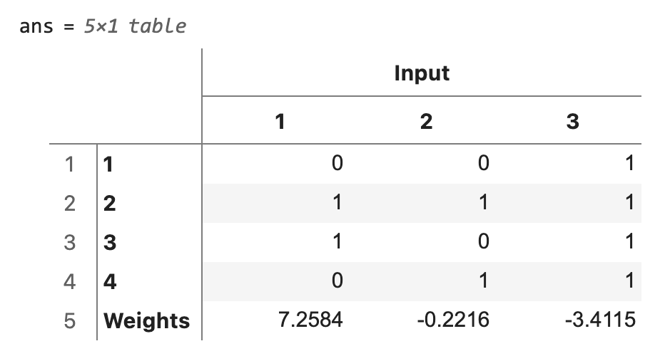
Weights w after training. If both input and output are 1, then we increase the weights. If the input is 1 and the output is 0, then we decrease the weights between input and output.
table(cat(1,x,w'),...
   'VariableNames',["Input"],...
   'RowNames',["1","2","3","4","Weights"])
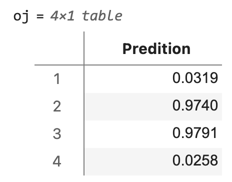
You can calculate each individual prediction using the input x, the weights w and the activation function sigfct. This is simply the sum of the input x weighted by w or, in other words, the inner product of x and w, passed to the activation function.
oj = table(sigfct(x*w),...
   'VariableNames',"Predition")
Here is a schematic display of our ANN with the three input nodes and the one single output node. The numerical values of the input x are the ones from the first sample / the first row [0 0 1] in x. The predicted output oj is the inner product of x and w, which yields –3.41, passed through the sigmoid function sigfct, which yields 0.0319, which in turn is very close to the expected output y of 0.
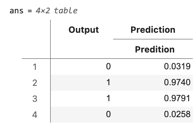
Output after training – You can see that the predicted value oj of the output y is very good.
table(y,oj,...
   'VariableNames',["Output","Prediction"])
Step 4 – Prediction
You can now use the trained ANN for prediction, e.g. to determine the Type 0 or 1 of any sample, such as
s = [0 0 1];
sigfct(s*w)

ans = 0.0319
As you can see, you get the expected result of a value close to zero.
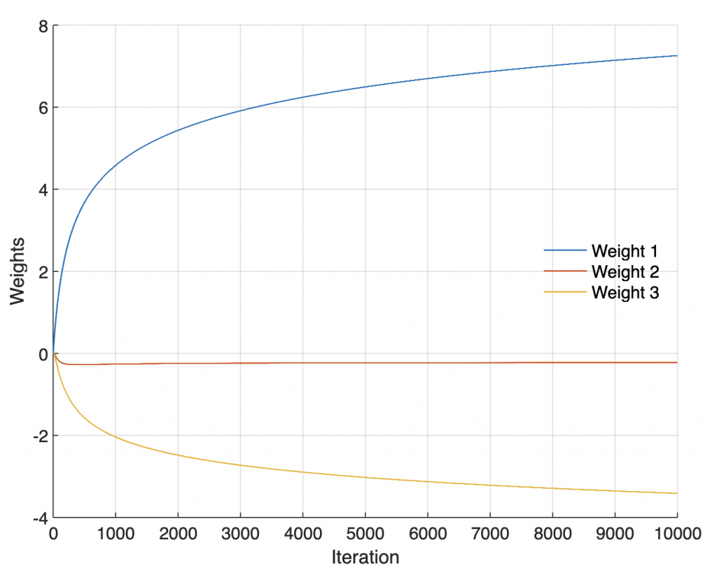
Step 5 – Graphical Display of the ANN Training
Graphical display of the weights w during the training.
axes('LineWidth',0.7,...
   'FontSize',12,...
   'XGrid','On',...
   'YGrid','On')
line(1:length(wi),wi,...
   'LineWidth',1)
xlabel('Iteration')
ylabel('Weights')
legend('Weight 1','Weight 2','Weight 3',...
   'FontSize',12,...
   'Location','East',...
   'Box','Off')
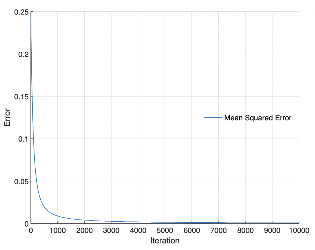
Graphical display of the mean squared error E during the training.
figure
axes('LineWidth',0.7,...
   'FontSize',12,...
   'XGrid','On',...
   'YGrid','On')
line(1:length(Ei),Ei,...
   'LineWidth',1)
xlabel('Iteration')
ylabel('Error')
legend('Mean Squared Error',...
   'FontSize',12,...
   'Location','East',...
   'Box','Off')
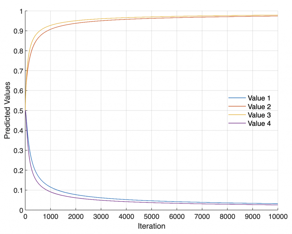
Graphical display of the predicted value oj of the output y during the training.
figure
axes('LineWidth',0.7,...
   'FontSize',12,...
   'XGrid','On',...
   'YGrid','On')
line(1:length(oji),oji,...
   'LineWidth',1)
xlabel('Iteration')
ylabel('Predicted Values')
legend('Value 1','Value 2','Value 3','Value 4',...
   'FontSize',12,...
   'Location','East',...
   'Box','Off')
Step 6 – The Activation Function
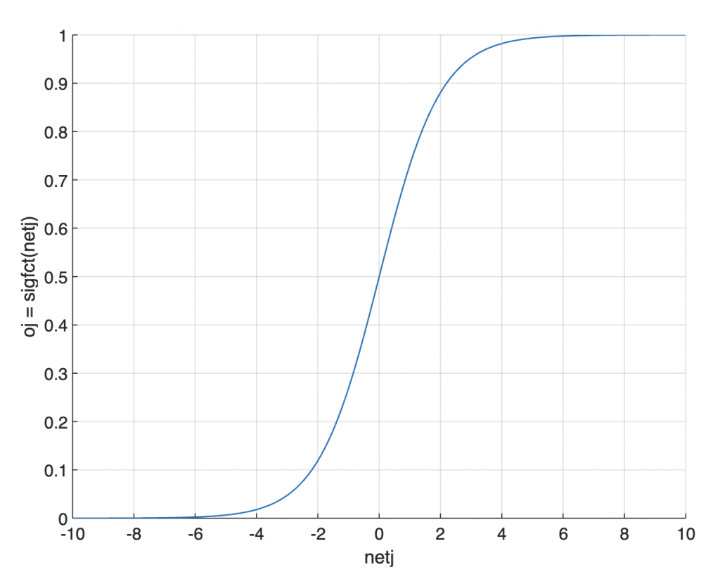
Sigmoid function sigfct. Please note that the input and output arguments x and y used here are not identical to the input and output x and y in the KNN example.
function y = sigfct(x)
   y = 1./(1+exp(-x));
end
Graphical display of sigmoid function.
xx = -10 : 0.1 : 10;
yy = sigfct(xx);

figure
axes('LineWidth',0.7,...
   'FontSize',12,...
   'XGrid','On',...
   'YGrid','On')
line(xx,yy,...
   'LineWidth',1)
xlabel('netj')
ylabel('oj = sigfct(netj)')
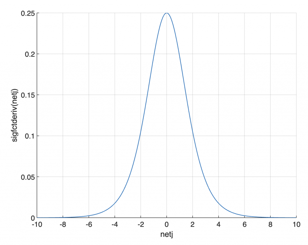
Sigmoid function’s derivative. There is a mistake in this function in the blog post by Trask (2015).
function y = sigfctderiv(x)
y = sigfct(x).*(1 - sigfct(x));
end
Graphical display of derivative of sigmoid function.
xx = -10 : 0.1 : 10;
yy = sigfctderiv(xx);

figure
axes('LineWidth',0.7,...
   'FontSize',12,...
   'XGrid','On',...
   'YGrid','On')
line(xx,yy,...
   'LineWidth',1)
xlabel('netj')
ylabel('sigfctderiv(netj)')
References
Trask, A. (2015) A neural network in 11 lines of Python (Part 1), I am Trask, A Machine Learning Craftsmanship Blog (Link).
Sanderson, G. (2017) Neural networks – The basics of neural networks, and the math behind how they learn (Link).
Daniel Sonnet (2022) Neuronale Netze kompakt, Vom Perceptron zum Deep Learning. Springer Vieweg, Berlin.