Here is a nice application of the script from MRES to count sand grains in microscopic images. In September 2013 a biologist from the National Museums of Kenya joint us on an expedition to the Suguta Valley in the Northern Kenya Rift. At that time hundreds of thousands of lesser flamingos left the Central Kenia Rift, especially from the Nakuru basin, and went to the Suguta Valley. The biologist started to count the flamingos, while I immediately thought about doing this automatically with a little MATLAB script.
We used a helicopter for moving around the largely inaccessible valley and I asked the pilot to move high enough to take air photos without disturbing the birds too much. Here is the example of how to use the script from Chapter 8.10 to count flamingos. Please read the chapter for the details about the script, which has not changed dramatically. You can get better results by modifying some of the parameters. We first read an image by typing
clear, clf
I1 = imread('flamingos_1.tif');
ix = 1063; iy = 622;
imshow(I1,'XData',[0 ix],'YData',[0 iy])
title('Original Image')
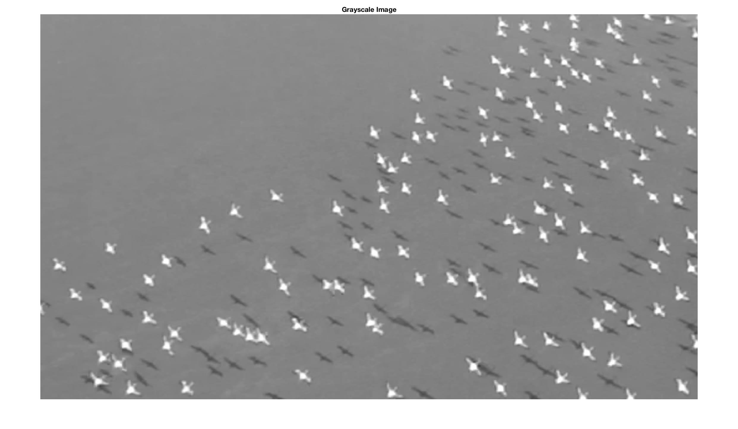
 We reject the color information of the image and convert I1 to grayscale using the function rgb2gray.
I2 = rgb2gray(I1);
imshow(I2,'XData',[0 ix],'YData',[0 iy])
title('Grayscale Image')
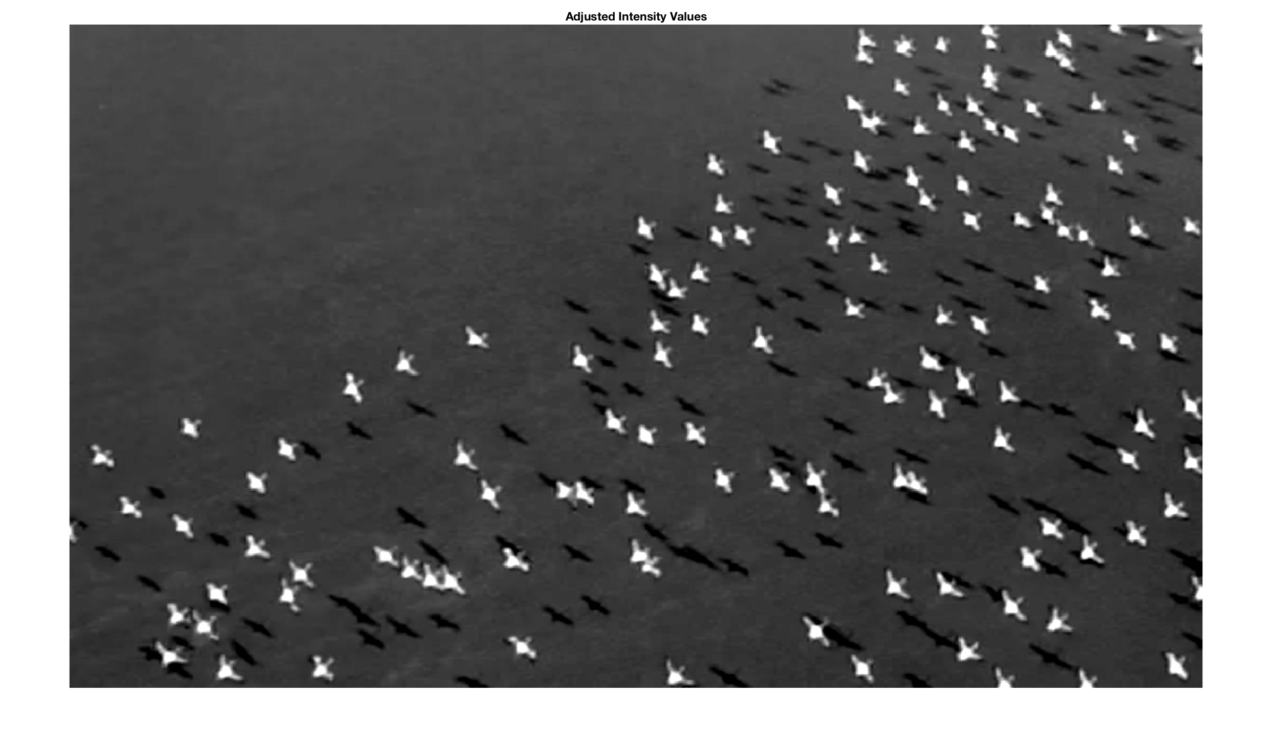
 This grayscale image I2 has a relatively low level of contrast. We therefore use the function imadjust to adjust the image intensity values.
I3 = imadjust(I2);
imshow(I3,'XData',[0 ix],'YData',[0 iy])
title('Adjusted Intensity Values')
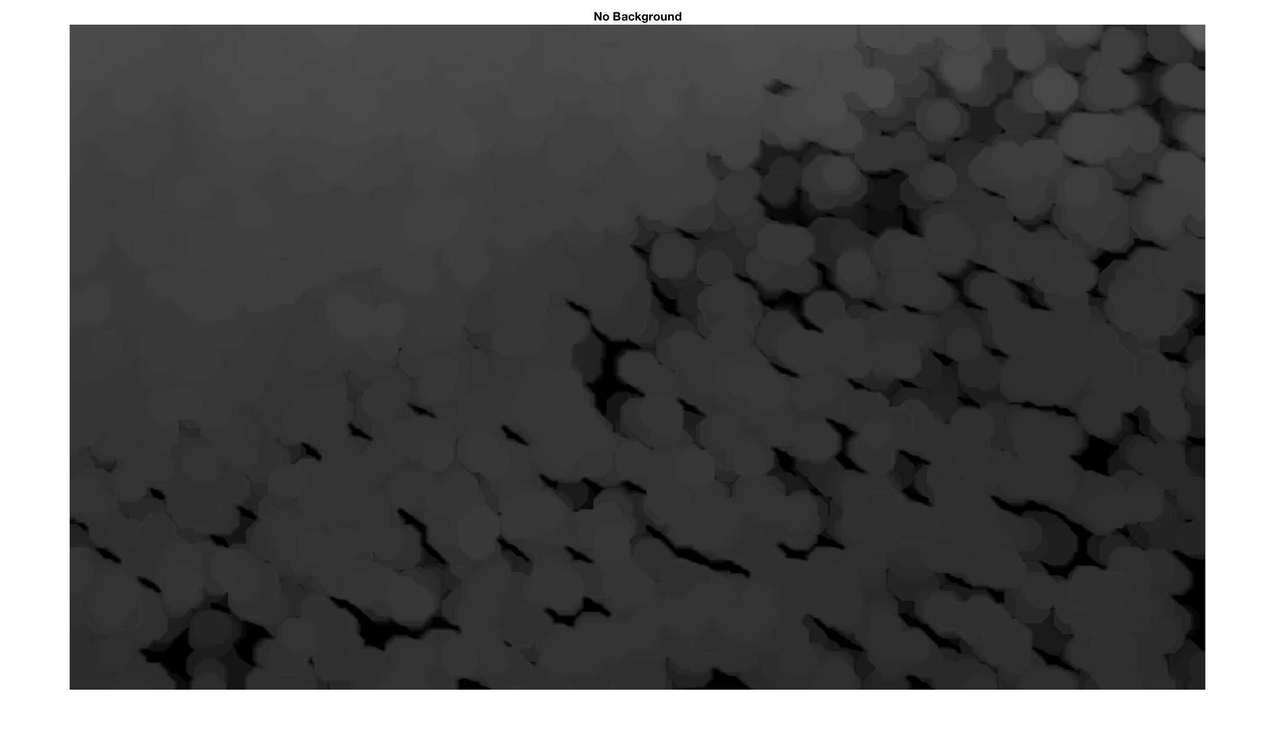
 We next determine the background of the I3 image, which means basically the texture of the black foil on which the grains are located. The function imopen(im,se) determines objects in an image im with a specific shape se (a flat structuring element such as a circular disk) and size (expressed as a specific number of pixels), as defined by the function strel.
I4 = imopen(I3,strel('disk',15));
imshow(I4,'XData',[0 ix],'YData',[0 iy])
title('No Background')
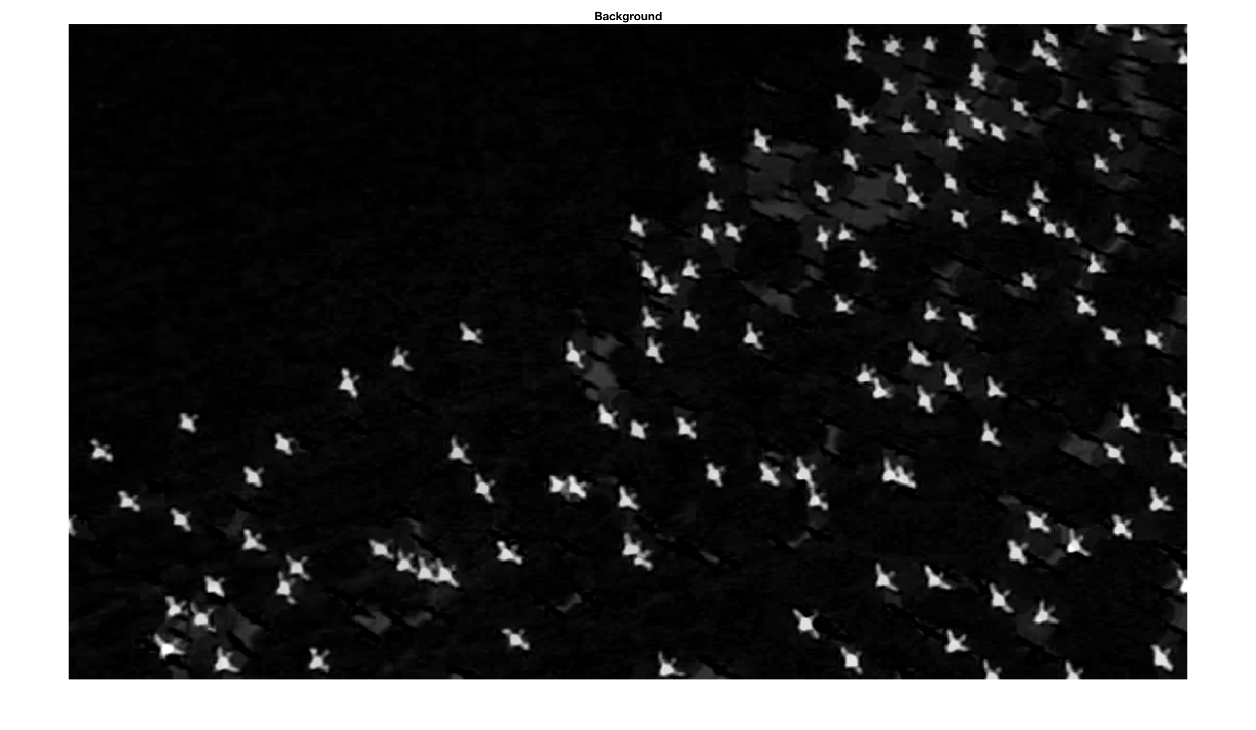
 We subtract the background-free image I4 from the original grayscale image I3 to observe the background I5 that has been eliminated.
I5 = imsubtract(I3,I4);
imshow(I5,'XData',[0 ix],'YData',[0 iy])
title('Background')
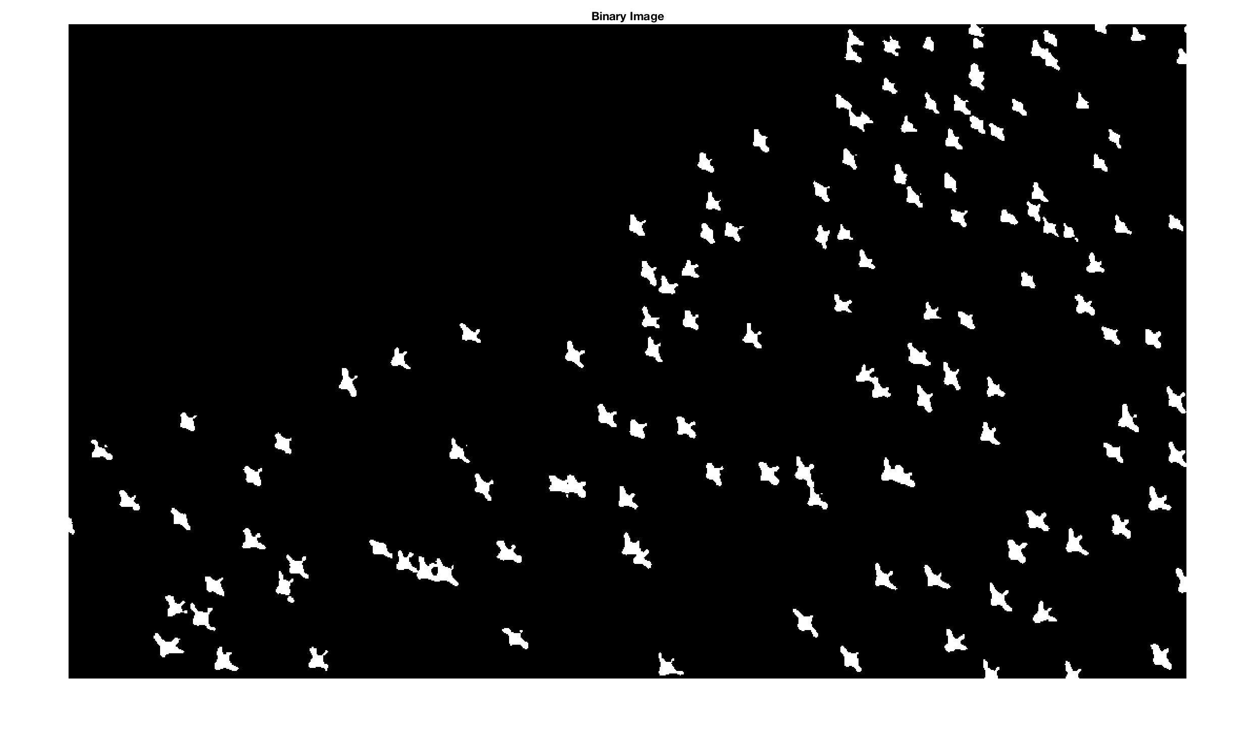
I6 = im2bw(I5,0.3);
imshow(I6,'XData',[0 ix],'YData',[0 iy])
title('Binary Image')
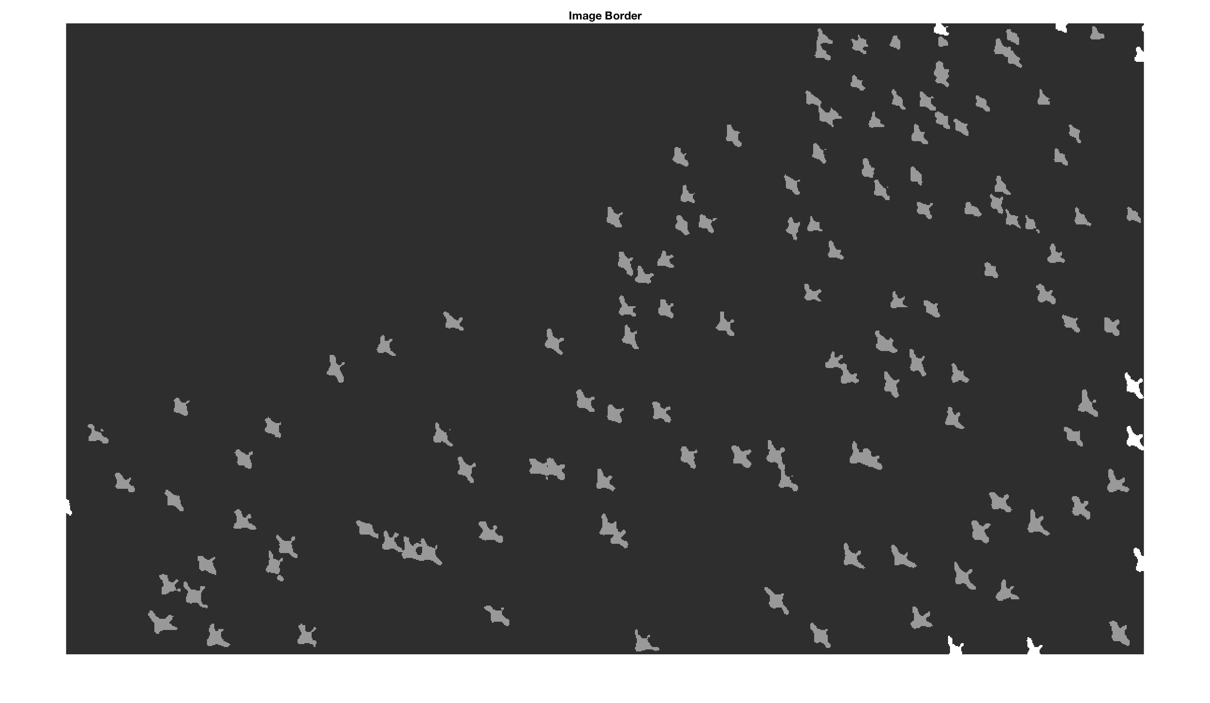
I7 = imclearborder(I6);
himage1 = imshow(I6,'XData',[0 ix],...
    'YData',[0 iy]); hold on
set(himage1, 'AlphaData', 0.7);
himage2 = imshow(imsubtract(I6,I7),...
    'XData',[0 ix],'YData',[0 iy]);
set(himage2, 'AlphaData', 0.4);
title('Image Border'), hold off
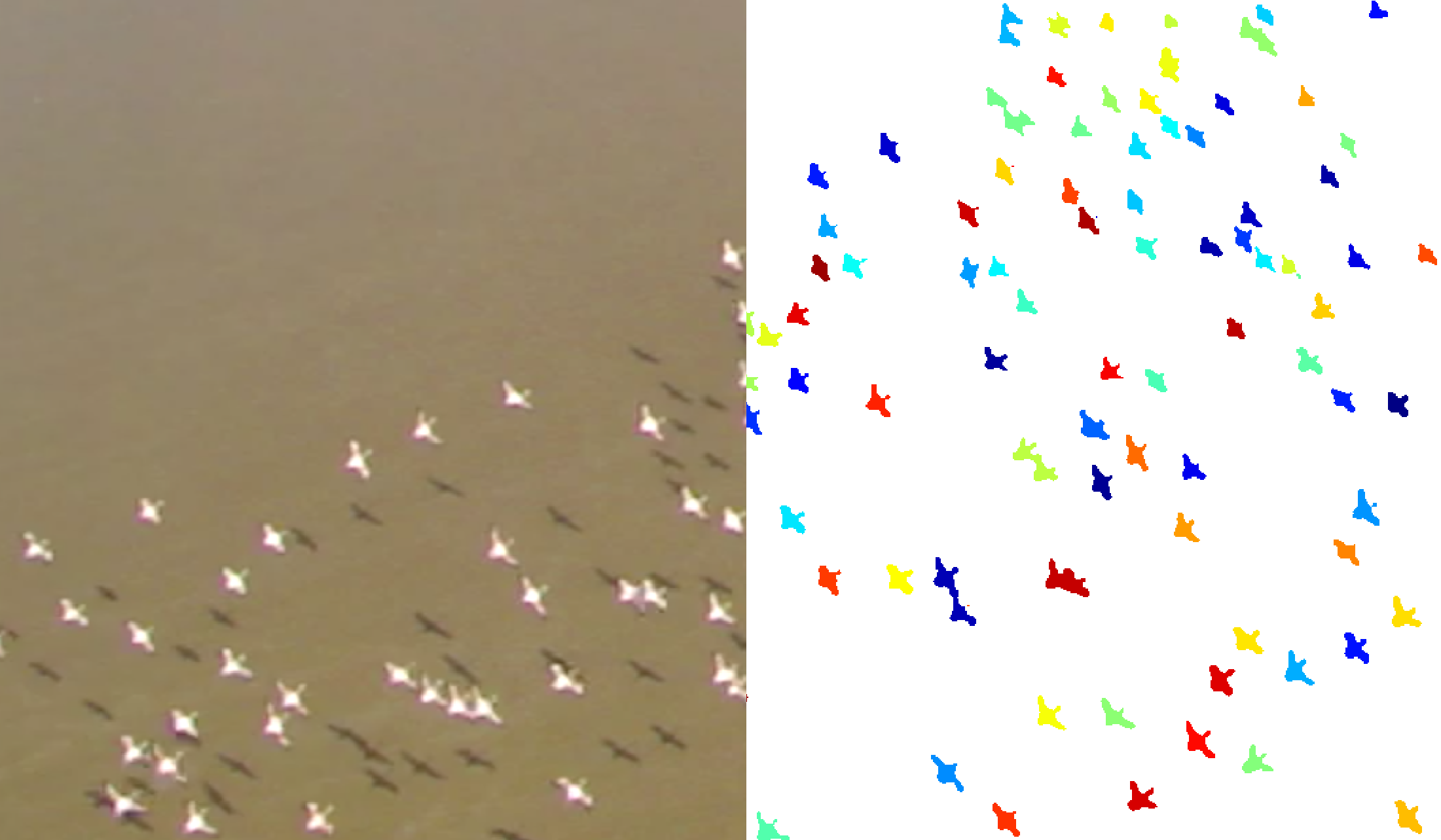
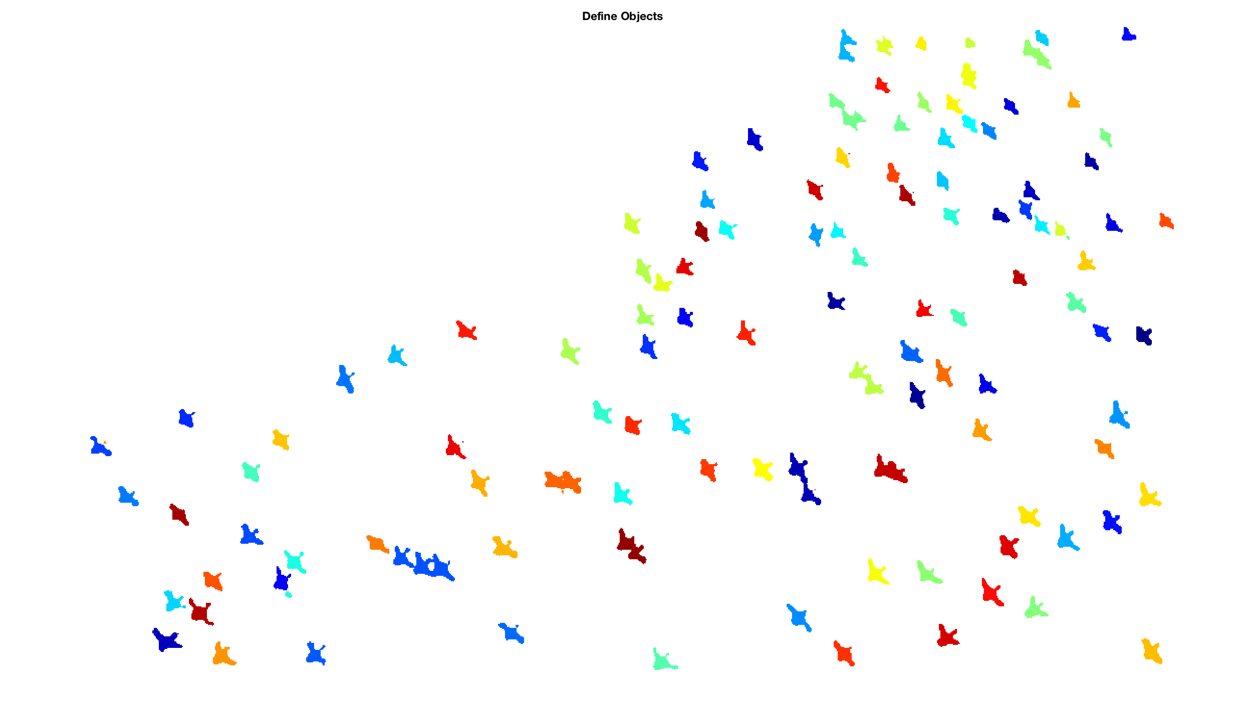
We then trace the boundaries using bwboundaries in a binary image where non-zero pixels belong to an object and zero pixels are background. By default, the function also traces the boundaries of holes in the I7 image. We therefore choose the option noholes to suppress the tracing of the holes. Function label2grb converts the label matrix L resulting from bwboundaries to an RGB image. We use the colormap jet, the zerocolor w for white, and the color order shuffle (which simply shuffles the colors of jet in a pseudorandom manner).
[B,I8] = bwboundaries(I7,'noholes');
imshow(label2rgb(I8,@jet,'w','shuffle'),...
    'XData',[0 ix],'YData',[0 iy])
title('Define Objects')
 The function bwlabeln is used to obtain the number of connected objects found in the binary image. The integer 8 defines the desired connectivity, which can be either 4 or 8 in two-dimensional neighborhoods. The elements of L are integer values greater than or equal to 0. The pixels labeled 0 are the background. The pixels labeled 1 make up one object, the pixels labeled 2 make up a second object, and so on.
[labeled,numObjects] = bwlabeln(I7,8);
numObjects
D = bwdist(~I8,'cityblock');
D = -D;
D(~I7) = -Inf;
I9 = watershed(D);
imshow(label2rgb(I9,@jet,'w','shuffle'),...
    'XData',[0 ix],'YData',[0 iy])
title('Watershed Segmentation')
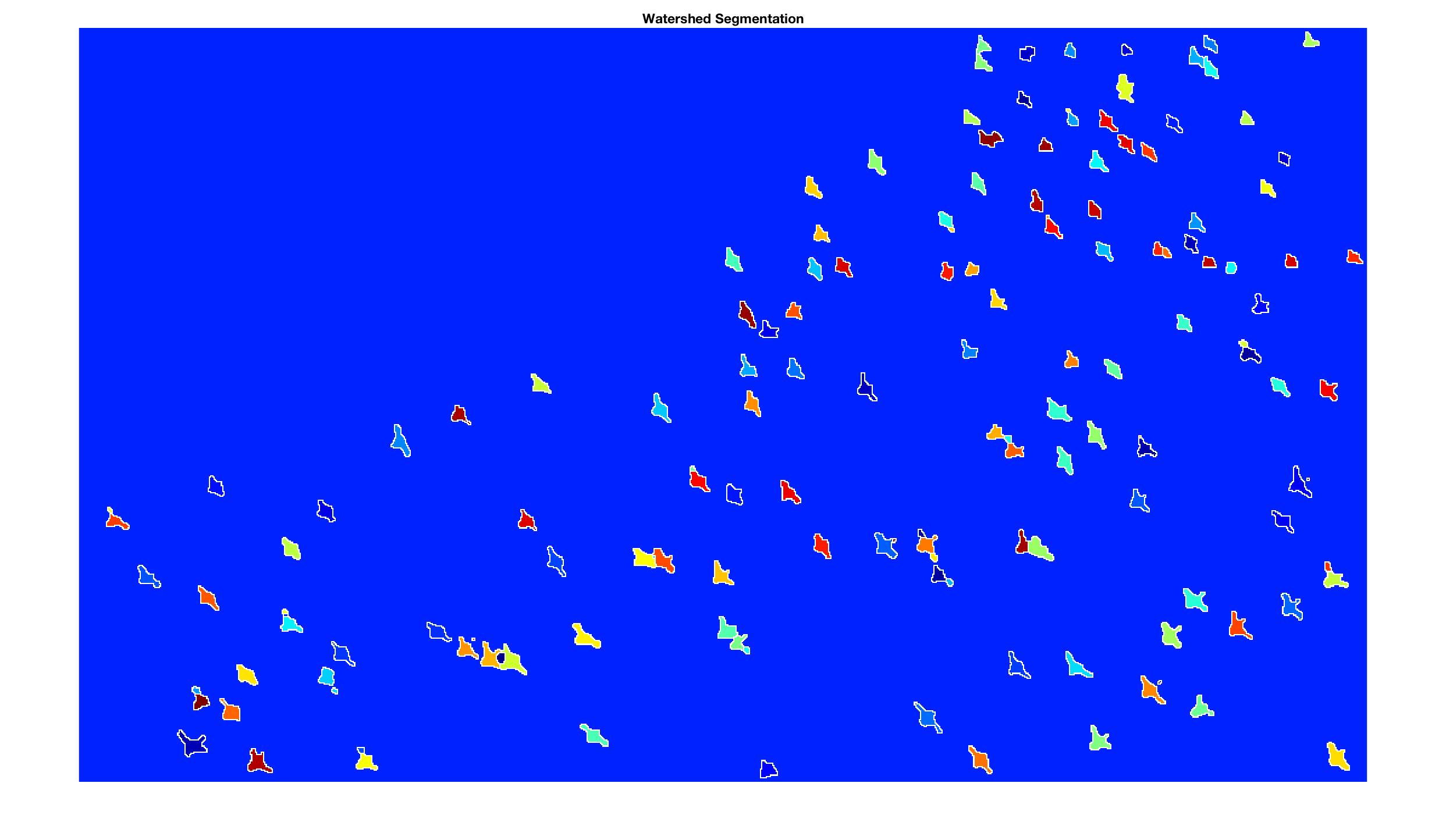
objects = sortrows(I9(:),1);
max(objects)
which yields the output ans = 152. This number of flamingos (152) is slightly higher than the manually counted number (122 + 8 incomplete flamingos) due to the effect of oversegmentation of the watershed algorithm. If this is a major problem when using segmentation to count objects in an image, the reader is referred to the book by Gonzalez, Woods and Eddins (2009) that describes marker-controlled watershed segmentation as an alternative method to avoid oversegmentation.
You can download the original image here.
References
Trauth, M.H. (2024) MATLAB Recipes for Earth Sciences – Sixth Edition. Springer International Publishing, 520 p.
Trauth, M.H. (2024) Python Recipes for Earth Sciences – Second Edition. Springer International Publishing, 450 p.