
In spectrometry—for example, in remote sensing—Gaussian filters or, because they are believed to cause less distortion, Savatzky-Golay filters are often used to improve the signal-to-noise ratio of spectra. Read here to find out how to do it better.
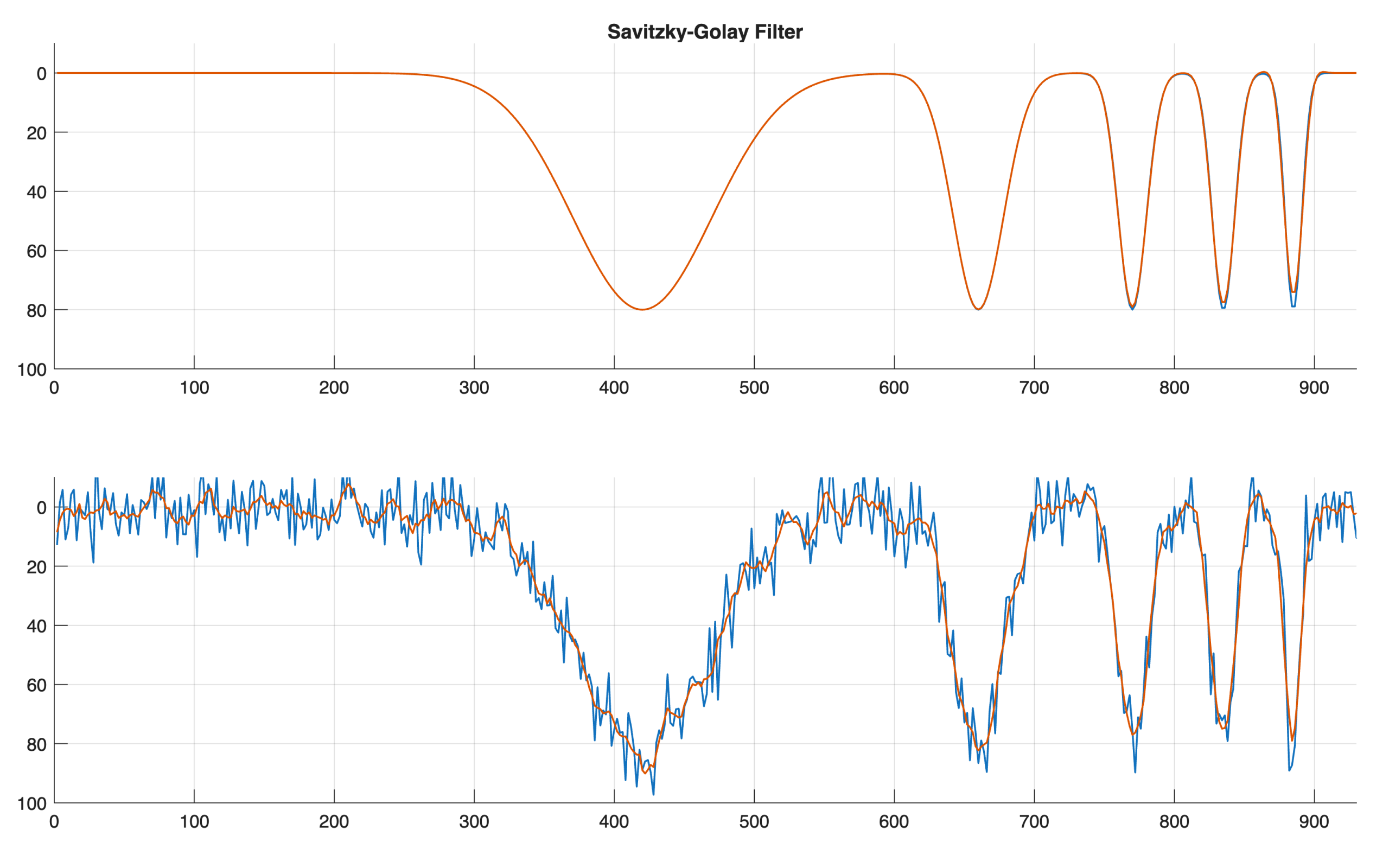
Gaussian filters are widely used in spectrometry to smooth spectra. Unfortunately, these filters have the undesirable property of reducing the depth of narrow absorption bands in reflectance spectra. For this reason, many users opt for Savitzky-Golay filters instead. The following example shows that while the effect is smaller when using Savitzky-Golay filters, it is still present. Therefore, users should opt for a recursive filter, such as a Butterworth low-pass filter, rather than non-recursive filters like Running Means, Gaussian or Savitzky-Golay filters. These filters leave the depth of the absorption bands unchanged up to a selectable width, while completely suppressing unwanted variations of narrower width.
Generate a Synthetic Time Series
The Savitzky-Golay filters (Savitzky and Golay, 1964) have achieved remarkable success compared to numerous similar, non-recursive filters. This success can be attributed to their inclusion in the highly influential book Numerical Recipes by Press et al. (1986).
On Page 647 of the book, Figure 14.8.1 presents a time series consisting of progressively narrower bumps with additive Gaussian noise. If the y-axis were inverted, this time series could serve as a model for a spectrum with progressively narrower absorption bands, where the y-axis represents reflectivity. In spectrometry, the depth and width of the bands are used to measure the amount of material absorbing at a specific wavelength. Filtering such a reflection spectrum to improve the signal-to-noise ratio should not alter the depth or width of the absorption bands, nor should it shift them along the x-axis, which represents the wavelength axis.
Unfortunately, the book does not provide the Fortran 77 code that generates this time series. However, it is now relatively easy to copy a screenshot of the top panel of the figure into ChatGPT, along with the prompt, Could you please write the MATLAB script to create a time series similar to the one shown on the figure?. After some testing, correction, and validation, the following MATLAB script was developed, generating a time series with characteristics similar to those of the time series in Figure 14.8.1, as shown in the uppermost panel.
clear, clc, close all

fs = 0.5;
t = 1/fs : 1/fs : 1000;

x = 80*exp(-(t-420).^2/(2*50^2));
x = x + 80*exp(-(t-660).^2/(2*18^2));
x = x + 80*exp(-(t-770).^2/(2*10^2));
x = x + 80*exp(-(t-835).^2/(2*8^2));
x = x + 80*exp(-(t-885).^2/(2*6^2));

xn = x + 8*randn(size(x));

figure('Position',[100 800 1200 800],...
    'Color',[1 1 1])
axes('Position',[0.1 0.5 0.8 0.3],...
    'XGrid','On',...
    'YGrid','On',...
    'XLim',[0 930],...
    'YLim',[-10 100],...
    'YDir','reverse')
line(t,x,...
    'LineWidth',1)
axes('Position',[0.1 0.1 0.8 0.3],...
    'XGrid','On',...
    'YGrid','On',...
    'XLim',[0 930],...
    'YLim',[-10 100],...
    'YDir','reverse')
line(t,xn,...
    'LineWidth',1)
Filtering Using Running Means
In certain fields running means are widely employed as a method for smoothing time series data. These running means, a specific instance of a moving average filter with identical weights, such as [0.2 0.2 0.2 0.2 0.2], represent a running mean. They have been readily available for decades due to their inclusion in numerous spreadsheet programs. In the provided example, we select a running mean over 11 values, ensuring that the filter has the same length as all the other filters discussed in this post. To generate the filter weights, we use the ones(11,1) function, and then we divide each weight by the sum of all the weights to ensure that the total is 1, eliminating any added variability.
b_rm = ones(11,1);
b_rm = b_rm/sum(b_rm);
x_rm = conv(x,b_rm,'same');
xn_rm = conv(xn,b_rm,'same');

figure('Position',[100 800 1200 800],...
    'Color',[1 1 1])
axes('Position',[0.1 0.5 0.8 0.3],...
    'XGrid','On',...
    'YGrid','On',...
    'XLim',[0 930],...
    'YLim',[-10 100],...
    'YDir','reverse')
line(t,x,...
    'LineWidth',1)
line(t,x_rm,...
    'LineWidth',1)
title('Running Mean')
axes('Position',[0.1 0.1 0.8 0.3],...
    'XGrid','On',...
    'YGrid','On',...
    'XLim',[0 930],...
    'YLim',[-10 100],...
    'YDir','reverse')
line(t,xn,...
    'LineWidth',1)
line(t,xn_rm,...
    'LineWidth',1)

As we observe, the depth of the absorption bands decreases as the bandwidth narrows, which is an undesirable characteristic of the filter in quantitative spectrometry. Moreover, these filters exhibit other undesirable properties, as evident from their characteristics in the frequency domain (or wavenumber domain) (see below, but also on page 313 in Trauth et al., 2025, and in the blog post Better Avoid Running Means).
[h_rm,w] = freqz(b_rm,1,512);

f = fs*w/(2*pi);

figure('Position',[100 800 800 600],...
    'Color',[1 1 1])
axes('Position',[0.1 0.1 0.35 0.8],...
    'XGrid','On',...
    'YGrid','On')
line(f,abs(h_rm),...
    'LineWidth',1)
title('Magnitude Response')
axes('Position',[0.55 0.1 0.35 0.8],...
    'XGrid','On',...
    'YGrid','On')
line(f,angle(h_rm),...
    'LineWidth',1)
title('Phase Response')
Filtering Using Gauss Filters
Gaussian filters are essentially moving average filters with filter weights whose time-dependent probability density function follows a Gaussian distribution. The sum of these weights must remain constant at one. Compared to a moving average with identical filter weights, the values of the weights are maximized at the center, at the peak of the Gaussian bell curve, and decrease symmetrically on both sides. This symmetry ensures that the position of the absorption bands remains unchanged.
b_gs = normpdf(-5:5,0,3);
b_gs = b_gs/sum(b_gs);
x_gs = conv(x,b_gs,'same');
xn_gs = conv(xn,b_gs,'same');

figure('Position',[100 800 1200 800],...
    'Color',[1 1 1])
axes('Position',[0.1 0.5 0.8 0.3],...
    'XGrid','On',...
    'YGrid','On',...
    'XLim',[0 930],...
    'YLim',[-10 100],...
    'YDir','reverse')
line(t,x,...
    'LineWidth',1)
line(t,x_gs,...
    'LineWidth',1)
title('Gauss Filter')
axes('Position',[0.1 0.1 0.8 0.3],...
    'XGrid','On',...
    'YGrid','On',...
    'XLim',[0 930],...
    'YLim',[-10 100],...
    'YDir','reverse')
line(t,xn,...
    'LineWidth',1)
line(t,xn_gs,...
    'LineWidth',1)

As we observe, the depth of the absorption bands fluctuates again as the bandwidth decreases, which is an undesirable characteristic of the filter in quantitative spectrometry. Similar to running means, these filters also exhibit other undesirable properties, as evident from their characteristics in the frequency domain (or wavenumber domain).
[h_gs,w] = freqz(b_gs,1,512);

f = fs*w/(2*pi);

figure('Position',[100 800 800 600],...
    'Color',[1 1 1])
axes('Position',[0.1 0.1 0.35 0.8],...
    'XGrid','On',...
    'YGrid','On')
line(f,abs(h_gs),...
    'LineWidth',1)
title('Magnitude Response')
axes('Position',[0.55 0.1 0.35 0.8],...
    'XGrid','On',...
    'YGrid','On')
line(f,angle(h_gs),...
    'LineWidth',1)
title('Phase Response')
Filtering Using Savitzky-Golay Filters
We apply a Savitzky-Golay filter of polynomial order 3 and frame length 11. As expected, the depth of the absorption bands decreases further, but to a lesser extent compared to the original filter.
[~,b_sg] = sgolay(3,11);
b_sg = b_sg(:,1);
x_sg = sgolayfilt(x,3,11);
xn_sg = sgolayfilt(xn,3,11);

figure('Position',[100 800 1200 800],...
    'Color',[1 1 1])
axes('Position',[0.1 0.5 0.8 0.3],...
    'XGrid','On',...
    'YGrid','On',...
    'XLim',[0 930],...
    'YLim',[-10 100],...
    'YDir','reverse')
line(t,x,...
    'LineWidth',1)
line(t,x_sg,...
    'LineWidth',1)
title('Savitzky-Golay Filter')
axes('Position',[0.1 0.1 0.8 0.3],...
    'XGrid','On',...
    'YGrid','On',...
    'XLim',[0 930],...
    'YLim',[-10 100],...
    'YDir','reverse')
line(t,xn,...
    'LineWidth',1)
line(t,xn_sg,...
    'LineWidth',1)
Similar to running means, these filters also have other undesirable properties, as evident when analyzing their characteristics in the frequency domain (or wavenumber domain).
[h_sg,w] = freqz(b_sg,1,512);

f = fs*w/(2*pi);

figure('Position',[100 800 800 600],...
    'Color',[1 1 1])
axes('Position',[0.1 0.1 0.35 0.8],...
    'XGrid','On',...
    'YGrid','On')
line(f,abs(h_sg),...
    'LineWidth',1)
title('Magnitude Response')
axes('Position',[0.55 0.1 0.35 0.8],...
    'XGrid','On',...
    'YGrid','On')
line(f,angle(h_sg),...
    'LineWidth',1)
title('Phase Response')
Filtering Using Butterworth Lowpass Filters
Now, we use a frequency-selective filter, specifically a lowpass filter designed using the Butterworth approach. Our goal is to remove noise from xn while preserving all wavelengths of the three absorption bands, which range from approximately 200 nm to 10 nm. These wavelengths correspond to wavenumbers of 1/200 nm^(-1) = 0.0050 nm^(-1) and 1/10 nm^(-1) = 0.1 nm^(-1). Consequently, the filter should eliminate wavelengths shorter than about 5 nm, which corresponds to a wavenumber of 1/5 nm^(-1) = 0.2 nm^(-1). We employ a Butterworth filter of the order 10, resulting in a filter length of 11, similar to the other filters used previously. Additionally, we set a cutoff wavelength of 5 nm or a cutoff wavenumber of 1/5 nm^(-1) = 0.2 nm^(-1).
[b_bw,a_bw] = butter(10,0.2/fs);
x_bw = filtfilt(b_bw,a_bw,x);
xn_bw = filtfilt(b_bw,a_bw,xn);

figure('Position',[100 800 1200 800],...
    'Color',[1 1 1])
axes('Position',[0.1 0.5 0.8 0.3],...
    'XGrid','On',...
    'YGrid','On',...
    'XLim',[0 930],...
    'YLim',[-10 100],...
    'YDir','reverse')
line(t,x,...
    'LineWidth',1)
line(t,x_bw,...
    'LineWidth',1)
title('Butterworth Filter')
axes('Position',[0.1 0.1 0.8 0.3],...
    'XGrid','On',...
    'YGrid','On',...
    'XLim',[0 930],...
    'YLim',[-10 100],...
    'YDir','reverse')
line(t,xn,...
    'LineWidth',1)
line(t,xn_bw,...
    'LineWidth',1)

These filters do not have any of the undesirable effects of the previous filters. They do not alter the amplitudes of the absorption bands within the passband of the filter. In contrast, they completely eliminate the amplitudes in the filter’s stopband. As you can observe from the magnitude and phase characteristics, these filters do not share the undesirable effects of the previous filters. They do not have zeros and do not exhibit the amplitude flipping as described below, which is also mentioned on page 313 in Trauth et al., 2025, and in the blog post titled Better Avoid Running Means. The phase response is not perfectly linear, indicating some distortion—albeit minimal—along the wavelength axis. However, this distortion is corrected by using a filter.
[h_bw,w] = freqz(b_bw,a_bw,512);

f = fs*w/(2*pi);

figure('Position',[100 800 800 600],...
    'Color',[1 1 1])
axes('Position',[0.1 0.1 0.35 0.8],...
    'XGrid','On',...
    'YGrid','On')
line(f,abs(h_bw),...
    'LineWidth',1)
title('Magnitude Response')
axes('Position',[0.55 0.1 0.35 0.8],...
    'XGrid','On',...
    'YGrid','On')
line(f,angle(h_bw),...
    'LineWidth',1)
title('Phase Response')
Comparing the Frequency Response of the Filters
The frequency response of the filters, including the magnitude response (the absolute value of the complex-valued frequency response) and the phase response (the angle of the complex-valued frequency response), offers deeper insights into how the filters affect the signal.
figure('Position',[100 800 800 600],...
    'Color',[1 1 1])
axes('Position',[0.1 0.1 0.35 0.8],...
    'XGrid','On',...
    'YGrid','On')
line(f,abs(h_rm),...
    'LineWidth',1)
line(f,abs(h_gs),...
    'LineWidth',1)
line(f,abs(h_sg),...
    'LineWidth',1)
line(f,abs(h_bw),...
    'LineWidth',1)
title('Magnitude Response')
legend('Running Mean',...
    'Gauss Filter',...
    'Savitzky-Golay Filter',...
    'Butterworth Lowpass Filter',...
    'Location','Northeast',...
    'Box','off')
axes('Position',[0.55 0.1 0.35 0.8],...
    'XGrid','On',...
    'YGrid','On')
line(f,angle(h_rm),...
    'LineWidth',1)
line(f,angle(h_gs),...
    'LineWidth',1)
line(f,angle(h_sg),...
    'LineWidth',1)
line(f,angle(h_bw),...
    'LineWidth',1)
title('Phase Response')
legend('Gauss',...
    'Savitzky-Golay',...
    'Butterworth',...
    'Location','Northeast',...
    'Box','off')

References
Press, W.H., Teukolsky, S.A., Vetterling, W.T., Flannery, B.P., 1986, 1992, 2001. Numerical Recipes in Fortran 77. Cambridge University Press, Cambridge. https://doi.org/10.2307/3616786 (Link)
Savitzky A., Golay, M.J.E. 1964. Analytical Chemistry, 36, 1627–1639. https://doi.org/10.1021/ac60214a047. (Link)
Trauth, M.H., 2025. MATLAB Recipes for Earth Sciences – Sixth Edition. Springer International Publishing, 567 p, https://doi.org/10.1007/978-3-031-57949-3. (Link)