On-screen digitizing is a widely-used image processing technique. While practical digitizer tablets exist in all formats and sizes, most people prefer digitizing vector data from the screen. Examples of this type of application include the digitizing of river networks and catchment areas on topographic maps, of the outlines of lithologic units on geological maps, of landslide distributions on satellite images, and of mineral grain distributions in microscopic images. The chapter on digitization is Section 8.7 in the MRES book. Here is an updated version of the section for use with MATLAB.
The digitizing procedure consists of the following steps. The image is first imported into the workspace. A coordinate system is then defined, allowing the objects of interest to be entered by moving a cursor or cross hair onto it and clicking the mouse button. The result is a two-dimensional array of xy data, such as longitudes and latitudes of the corner points of a polygon, or the coordinates of the objects of interest in a particular area.
The function ginput included in the standard MATLAB toolbox allows graphical input from the screen, using a mouse. It is generally used to select points, such as specific data points, from a figure created by an arbitrary graphics function such as plot. The function ginput is often used for interactive plotting, that is, the digitized points appear on the screen after they have been selected. The disadvantage of the function is that it does not provide coordinate referencing on an image. We therefore use a modified version of the function, which allows an image to be referenced to an arbitrary rectangular coordinate system. Save the following code for this modified version of the function ginput in a text file minput.m.
function y = minput(x)

xmin = input('Specify xmin! ');
xmax = input('Specify xmax! ');
ymin = input('Specify ymin! ');
ymax = input('Specify ymax! ');
B = imread(x);
a = size(B,2); b = size(B,1);
imshow(B);
disp('Click on ll and ur corner, then <return>')
[xcr,ycr] = ginput;
XMIN=xmin-((xmax-xmin)*xcr(1,1)/(xcr(2,1)-xcr(1,1)));
XMAX=xmax+((xmax-xmin)*(a-xcr(2,1))/(xcr(2,1)-xcr(1,1)));
YMIN=ymin-((ymax-ymin)*ycr(1,1)/(ycr(2,1)-ycr(1,1)));
YMAX=ymax+((ymax-ymin)*(b-ycr(2,1))/(ycr(2,1)-ycr(1,1)));
disp('Click on points to digitize, then <return>')
[xcoord,ycoord] = ginput;
Xcoord = XMIN + ((XMAX-XMIN)*xcoord / size(B,2));
Ycoord = YMIN + ((YMAX-YMIN)*ycoord / size(B,1));
y(:,1) = Xcoord; y(:,2) = Ycoord;
The function minput has four stages. In the first stage the user enters the limits of the coordinate axes as reference points for the image. The image is then imported into the workspace and displayed on the screen. The third stage uses ginput to define the upper left and lower right corners of the image. In the fourth stage the relationship between the coordinates of the two corners on the figure window and the reference coordinate system is then used to compute the transformation for all of the digitized points.
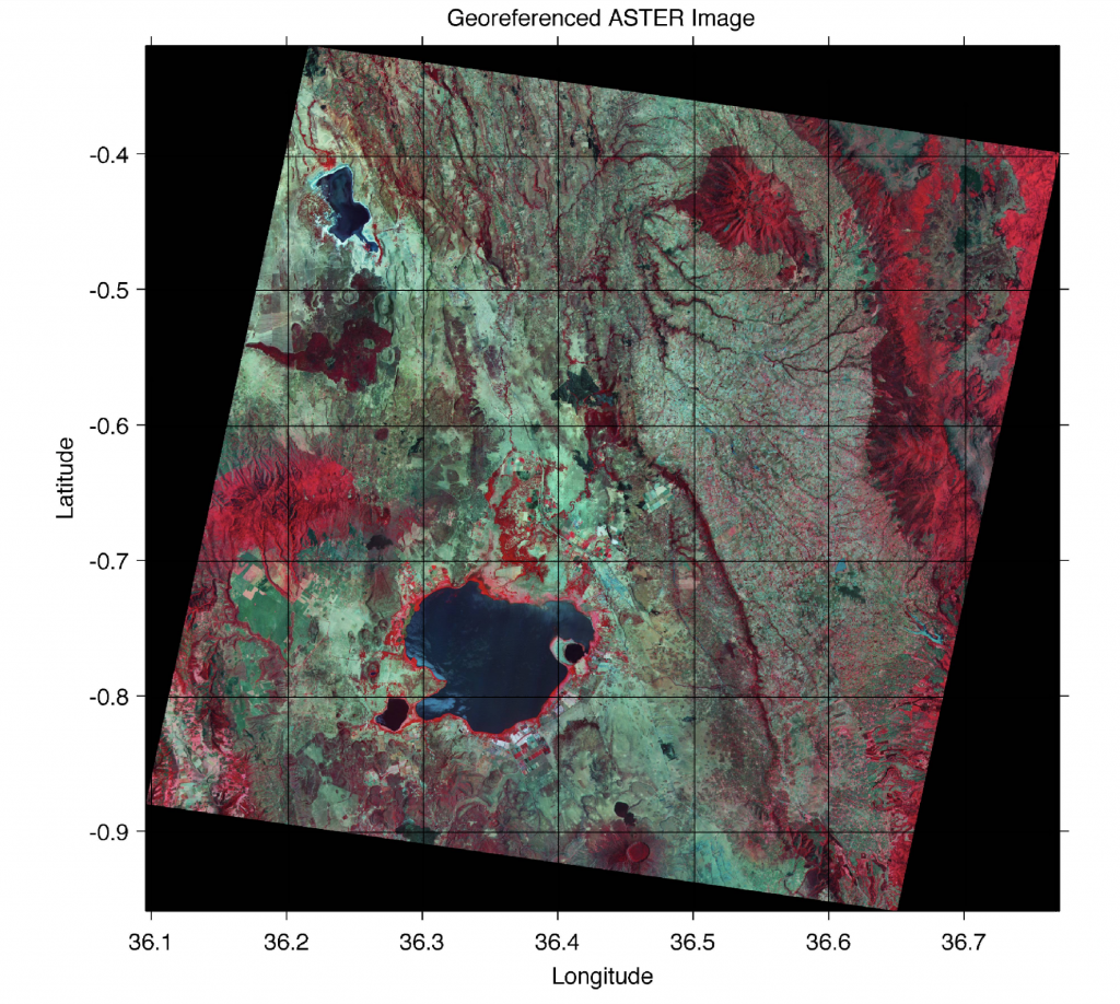
As an example we use the image stored in the file naivasha_georef.jpg and digitize the outline of Lake Naivasha in the center of the image. We activate the new function minput from the Command Window using the commands
clear

data = minput('naivasha_georef.jpg')
The function first asks for the coordinates of the limits of the x-axis and the y-axis, for the reference frame. We enter the corresponding numbers and press return after each input.
Specify xmin! 36.1
Specify xmax! 36.77
Specify ymin! -0.88
Specify ymax! -0.4
The function then reads the file naivasha_georef.jpg and displays the image. We ignore the warning
Warning: Image is too big to fit on screen;
displaying at 33%
and wait for the next response
Click on ll and ur corner, then <return>
The image window can be scaled according to user preference. Clicking on the lower left and upper right corners of the rotated satellite image (not the corners of the underlying black background) defines the dimensions of the image. These changes are registered by pressing return. The routine then references the image to the coordinate system and waits for the input of the points we wish to digitize from the image.
Click on points to digitize, then <return>
We can now digitize, for example, the outline of the lake, tectonic faults or tuff cones. We finish the input by again pressing return. The xy coordinates of our digitized points are now stored in the variable data. We can now use these vector data for other applications.
References
Trauth, M.H. (2021) MATLAB Recipes for Earth Sciences – Fifth Edition. Springer International Publishing, 517 p., ISBN 978-3-030-38440-1. (MRES)


