
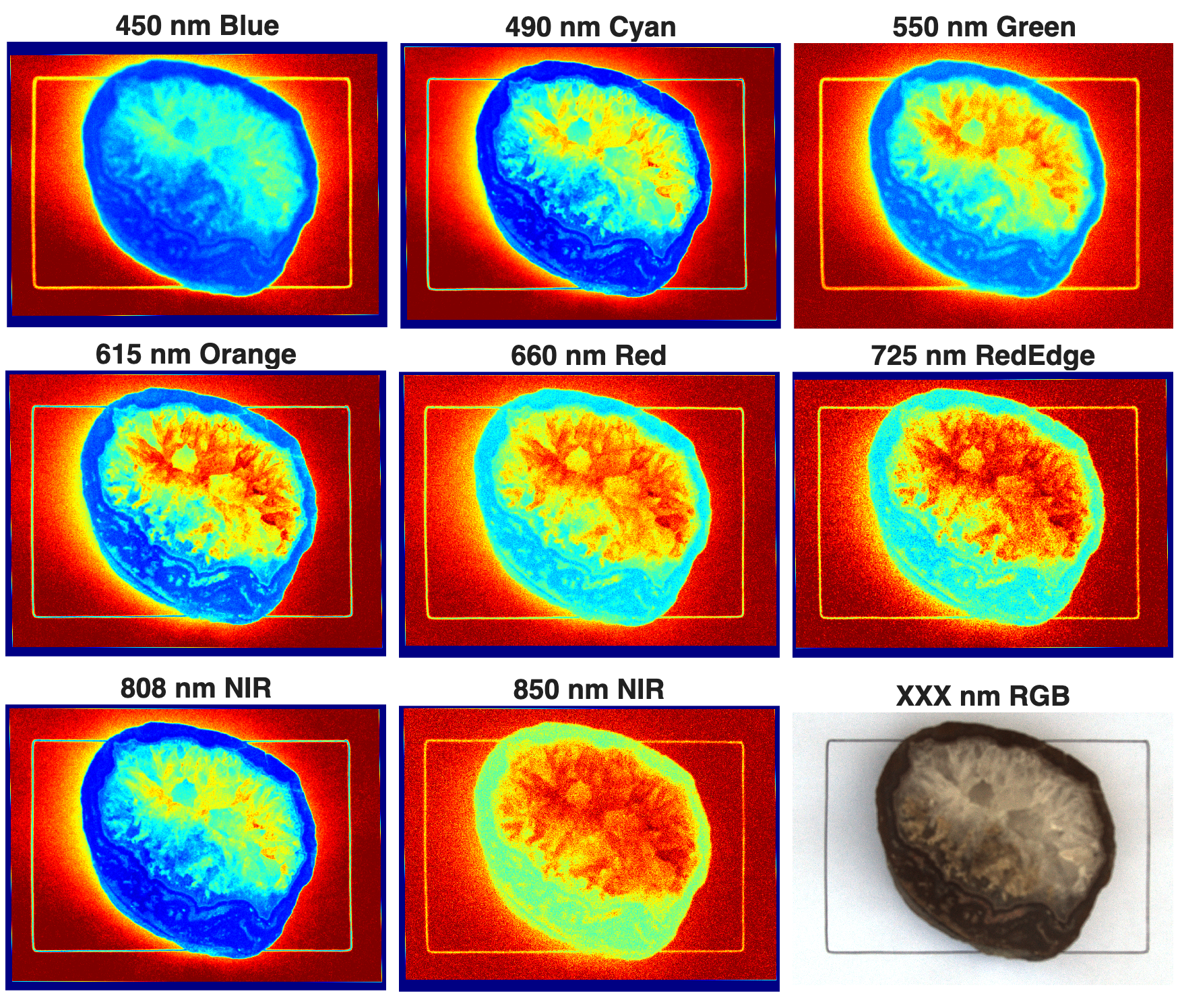
Multispectal imaging captures images across multiple spectral bands. Here is a MATLAB example where eight different spectral bands in visible light and near infrared show differences in a rock sample that are invisible to the human eye.
In an earlier post, I described how to process images taken with the new MAPIR Survey3 spectral cameras using MATLAB. A few years ago, and thanks to the ongoing support of MathWorks Inc. through their Curriculum Development Program, I now have four Survey2 and two Survey3 cameras. In the following MATLAB script, the data from these cameras is combined into a multispectral data set despite the different dimensions of the images.
Image acquisition is performed as described in the earlier post. Minor differences between the 16-megapixel Survey2 and 12-megapixel Survey3 cameras are compensated for in the respective scripts, which, like the data, can be found in the download area at the end of the blog post.
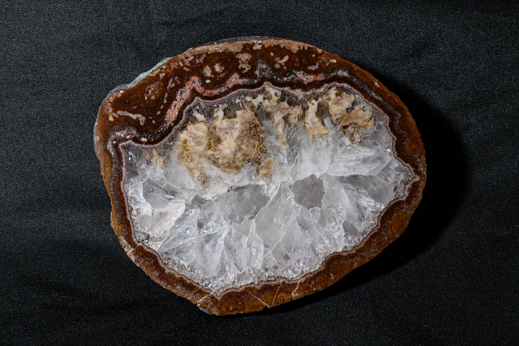
The actual sample is a sawn and polished agate druse sampled from a 290-million-year (Permian) basalt (so-called melaphyr) from Waldhambach, southern Germany. It consists mainly of colorless crystalline quartz in the center, surrounded by several layers of agate, usually colored red due to Fe oxide admixtures, with small cavities also filled with quartz.
First, we load the image data from the .mat files, which were previously generated in the scripts according to the older post.
load mapirsurvey2_660_850.mat
load mapirsurvey2_450.mat
load mapirsurvey3_725.mat
load mapirsurvey3_615_490_808.mat
load mapirsurvey2_rgb.mat
load mapirsurvey2_550.mat
Then we define the variables image1 to image9 for the individual wavelengths or the RGB image:
image1 = mapirsurvey2_450;                % 450 nm
image2 = mapirsurvey3_615_490_808(:,:,2); % 490 nm
image3 = mapirsurvey2_550;                % 550 nm
image4 = mapirsurvey3_615_490_808(:,:,1); % 615 nm
image5 = mapirsurvey2_660_850(:,:,1);     % 660 nm
image6 = mapirsurvey3_725;                % 725 nm
image7 = mapirsurvey3_615_490_808(:,:,3); % 808 nm
image8 = mapirsurvey2_660_850(:,:,3);     % 850 nm
image9 = mapirsurvey2_rgb;                % RGB
We can initially display the individual images in a mosaic.
figure('Position',[50 800 800 800])
tiledlayout(3,3, ...
   'TileSpacing','compact');
nexttile, imshow(image1), title('450 nm Blue')
nexttile, imshow(image2), title('490 nm Cyan')
nexttile, imshow(image3), title('550 nm Green')
nexttile, imshow(image4), title('615 nm Orange')
nexttile, imshow(image5), title('660 nm Red')
nexttile, imshow(image6), title('725 nm RedEdge')
nexttile, imshow(image7), title('808 nm NIR')
nexttile, imshow(image8), title('850 nm NIR')
nexttile, imshow(image9), title('XXX nm RGB')
Next, we prepare the registration of the images, i.e., we define the type of transformation to make the images compatible.
% Registration
[optimizer,metric] = imregconfig('monomodal');
In our example, we use image3 as the reference image. You can also use other images as reference images, but in our example, this meant that referencing did not work in all examples. Alternatively, you could achieve this by adjusting the parameters in imregconfig.
refimage = image3;
We then carry out the actual transformation of all images. The results are also displayed in the script in the download area.
image1_reg = imregister(image1,refimage,...
   'affine',optimizer,metric);
image2_reg = imregister(image2,refimage,...
   'affine',optimizer,metric);
image3_reg = imregister(image3,refimage,...
   'affine',optimizer,metric);
image4_reg = imregister(image4,refimage,...
   'affine',optimizer,metric);
image5_reg = imregister(image5,refimage,...
   'affine',optimizer,metric);
image6_reg = imregister(image6,refimage,...
   'affine',optimizer,metric);
image7_reg = imregister(image7,refimage,...
   'affine',optimizer,metric);
image8_reg = imregister(image8,refimage,...
   'affine',optimizer,metric);
image9_reg = imregister(image9(:,:,1),refimage,...
   'affine',optimizer,metric);
We concatenate the now congruent images with the dimensions 935×1315 into a single variable image.
image = cat(3,...
   image1_reg,...
   image2_reg,...
   image3_reg,...
   image4_reg,...
   image5_reg,...
   image6_reg,...
   image7_reg,...
   image8_reg,...
   image9_reg);
Finally, we put all the matching images of the individual wavelengths back together in a mosaic.
cmap = 'jet';
figure('Position',[50 800 800 800])
tiledlayout(3,3, ...
'TileSpacing','compact');
nexttile, imshow(image1_reg)
title('450 nm Blue')
colormap(cmap)
nexttile, imshow(image2_reg)
title('490 nm Cyan')
colormap(cmap)
nexttile, imshow(image3_reg)
title('550 nm Green')
colormap(cmap)
nexttile, imshow(image4_reg)
title('615 nm Orange')
colormap(cmap)
nexttile, imshow(image5_reg)
title('660 nm Red')
colormap(cmap)
nexttile, imshow(image6_reg)
title('725 nm RedEdge')
colormap(cmap)
nexttile, imshow(image7_reg)
title('808 nm NIR')
colormap(cmap)
nexttile, imshow(image8_reg)
title('850 nm NIR')
colormap(cmap)
nexttile, imshow(image9)
title('XXX nm RGB')
colormap(cmap)

print -dpng -r300 mapirsurvey3all.png
you can clearly see that the red areas on the rock sample reflect more strongly in the orange wavelength range, while the quartz reflects more strongly in the cyan range, as expected. As already seen in the example of the OCN image in the older post, you can clearly see the differences between the blue and red tones in the image, for example.
Downloads
Download the MATLAB script and the image data (363 MB)
References
Trauth, M.H. (2025) MATLAB Recipes for Earth Sciences – Sixth Edition. Springer International Publishing, 567 p.
Trauth, M.H. (2021) Signal and Noise in Geosciences, MATLAB Recipes for Data Acquisition in Earth Sciences. Springer International Publishing, 544 p.