
Thanks to the ongoing support of MathWorks Inc. through their Curriculum Development Program, I was able to purchase two additional spectral cameras. The MAPIR Survey2 cameras are no longer available. They have been replaced by the Survey3, which has slightly different features. Here is an example of how to import and process the RAW images in MATLAB.
In an earlier post, I described how to process images taken with MAPIR Survey2 spectral cameras using MATLAB. These cameras are now manufactured by MAPIR Inc., formerly known as Peau Productions Inc. In the European Union and the United Kingdom, the cameras are distributed by SeeSense. SeeSense is run by Jana and Nigel Paine based in the Slovak Republic and an office in Northamptonshire in the United Kingdom. Both were extremely friendly and helpful, answering my questions quickly and thoroughly. The order through the university procurement department went smoothly and quickly.
The new Survey3 has a 16 bit Sony Exmor R IMX117 12 megapixel Bayer RGGB sensor with 4,000 x 3,000 pixels, whereas the old Survey2 have a 16 bit Sony Exmor IMX206 16MP 16 megapixel Bayer RGGB sensor with 3,456×4,608 pixels. I purchased the OCN (orange, cyan, near infrared or NIR) and RE (red-edge) filter options of the Survey3 in addition to the four Survey2 cameras with NDVI Red+NIR (650 and 850 nm), Blue (450 nm), Green (550 nm) and Visible Light RGB (~370–650 nm).
Both cameras are, similar to my older Survey2 cameras, the wide-angle lens version; hence, I bought Survey3W cameras with an 87-degree horizontal angle of view and an 81 cm default minimum focus distance. The cameras are therefore not very suitable for close-ups of minerals and rocks, but even at a distance of 22 cm, usable (albeit not entirely sharp) images can be obtained, as we see below. I took the photos outdoors, but in the shade, using a tripod, automatic white balance, multi-field metering for focus, and an exposure time of 1/125 s. I experimented with other settings but could not see any improvement.
The example below uses the three spectral bands of the OCN camera, namely orange (615 nm wavelength, 42 nm band width), cyan or blue/green (490 nm, 36 nm), and near-infrared or near-infrared (808 nm, 50 nm). The three wavelengths are therefore different from those of the three types of cones in the human eye, which have maximum sensitivity at 420 nm, 530 nm, and 560 nm, and with a much wider bandwidth. Another difference to the human eye is that, apart from the Bayer mosaic, color sensitivity is largely evenly distributed across the 12 megapixels.
The new Survey3 cameras have additional advantages over the old Survey3 cameras. For example, they finally have a thread for attaching them to a tripod. I attached the old cameras to the tripod using a clamp mount for smartphones. Another new feature is the discontinuation of one of the three control buttons. Instead, the Survey3 has a touchscreen, which is difficult to use due to the small size of the 2-inch display. In my experiments, it took several attempts to access the camera settings (bottom left) or the recording settings (bottom right).
The cameras are fairly easy to use, provided you have managed to gather all the necessary information, which is scattered across the MAPIR website. There is no comprehensive manual, just a very brief guide in a leaflet that gives a quick overview of the software. I have therefore written a one-page instruction manual for both cameras, Survey2 and Survey3:
Survey 2 Manual (Trauth, 2019)
Survey 3 Manual (Trauth, 2025)
As with many other manufacturers of specialized hardware, a major problem is that they offer compatible software. The software generates additional costs, and it is easy to see that the company makes more profit from selling the software than from selling the hardware. The problem, however, is that important information about the nature of the data is not provided or is only provided in a hidden manner.
When using the camera, it is important to ensure that it is completely switched off before disconnecting any cables or removing the memory card. Failure to do so will cause the camera to malfunction, making it particularly difficult to switch on and off and operate. At first, I was too impatient and was tempted to complain to support about the unreliable hardware and software, until I finally took the time to read the user manual with the important note.
First, we read the file information from the header of the RAW file and define the variables row and col for the dimensions of the image using
clear, clc, close all

filename = '2025_0811_091718_003.RAW';
inf = rawinfo(filename);
row = inf.CFAImageSize(:,1);
col = inf.CFAImageSize(:,2);
Then we load the actual data from the RAW file. According to the message from Ethan Hall from MAPIR Inc. and the information provided on the Mapir website, only 12 bits are used from the 16 bit Sony Exmor R IMX117 12MP Bayer RGGB sensor. We use ubit12=>uint16 to store the 12 bits in a uint16 array before we transpose the image.
id = fopen(filename);
I1 = fread(id,[col,row],'ubit12=>uint16');
I1 = I1';
We then demosaic the RGGB Bayer pattern encoded image to a truecolor (RGB) image using gradient-corrected linear interpolation:
I2 = demosaic(I1,'rggb');
The 16 bit image has a [6 490] range of values, the full 16 bit range is [0 65535] and therefore displaying the image with imshow yields a very dark image. This is because the image is actually a 12-bit image with a value range of [0 4096]. When we display the 16-bit image with imshow, the function assumes a uint16 value range of [0 65535] and produces a very dark image. One way to solve this problem is to scale the value range of the image to the full uint16 value range:
min(I2(:))
max(I2(:))
I3 = rescale(I2);
For all types of images, it is important to perform color correction, usually in the form of white balance. For calibrating MAPIR images, especially those taken by drones, MAPIR provides a reference target, which is, however, somewhat too large for capturing rocks and minerals. For all types of images, it is important to perform color correction, usually in the form of white balance. For calibrating MAPIR images, especially those taken by drones, MAPIR provides a reference target, which is, however, somewhat too large for capturing rocks and minerals. I have the slightly older Reflectance Standard Calibration Target; the new model comes in a waterproof outer case.
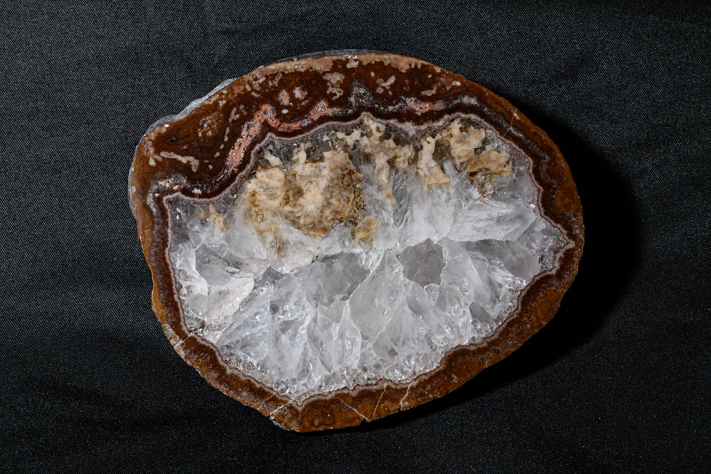
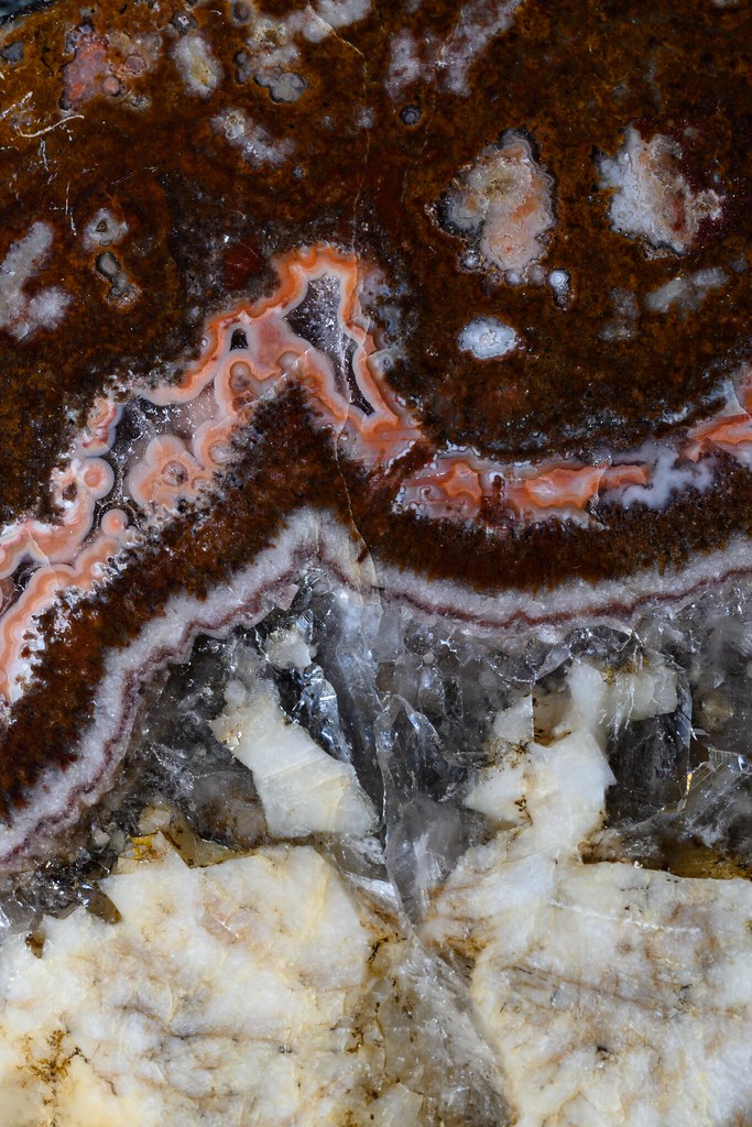
The method used for white balance depends on the application, especially if the reflectance values are to be used quantitatively, for example, in combination with images from other MAPIR cameras. In the following example, we took the photos using the camera’s automatic white balance. However, we also performed a white balance for each channel individually, using a rectangular area on the white background on which the rock sample is lying as a reference. The actual sample is a sawn and polished agate druse sampled from a 290-million-year (Permian) basalt (so-called melaphyr) from Waldhambach, southern Germany. It consists mainly of colorless crystalline quartz in the center, surrounded by several layers of agate, usually colored red due to Fe oxide admixtures, with small cavities also filled with quartz.
To perform a white balance, we first select a rectangular area that is known to be white. If we scale the image to the uint16 value range as described above, it appears very green in the RGB display. Remember that this is not an RGB image, but an OCN image, which means that what appears green is actually more cyan, for example.
imshow(I3), title('Mark rectangular white area')
roi = drawrectangle;
position = roi.Position;
position = round(position);
We then perform white balance separately for each channel by scaling the entire image so that the rectangular reference area is actually white, i.e., has a uint16 value of 65535. To do this, we first calculate the average value of the pixels in the reference area, divide the values of all pixels by this average value, and multiply the result by 65535. To ensure that these operations are not affected by the limitations of integer (uint16) data, we temporarily convert them to the single data type.
B_white = mean2(I3(position(2)-...
   position(4):position(2),...
   position(1):position(1)+...
   position(3),1));
I4(:,:,1) = uint16(single(I3(:,:,1))...
   *single(2^16)/B_white);

B_white = mean2(I3(position(2)-...
   position(4):position(2),...
   position(1):position(1)+...
   position(3),2));
I4(:,:,2) = uint16(single(I3(:,:,2))...
   *single(2^16)/B_white);

B_white = mean2(I3(position(2)-...
   position(4):position(2),...
   position(1):position(1)+...
   position(3),3));
I4(:,:,3) = uint16(single(I3(:,:,3))...
   *single(2^16)/B_white);
As a further step, we could rectify the image. To do this, we select the UL, LL, UR, and LR points of the rectangle and press the Return key. The following lines of code perform a projective transformation, which can also be replaced by other types of transformation, e.g. affine.
imshow(I4)
title('Click UL, LL, UR, LR, then press return')
movingpoints = ginput;

dx = (movingpoints(3,1)+movingpoints(4,1))/2- ...
   (movingpoints(1,1)+movingpoints(2,1))/2;
dy = (movingpoints(2,2)+movingpoints(4,2))/2- ...
   (movingpoints(1,2)+movingpoints(3,2))/2;

fixedpoints(1,:) = [0 0];
fixedpoints(2,:) = [0 dy];
fixedpoints(3,:) = [dx 0];
fixedpoints(4,:) = [dx dy];

tform = fitgeotrans(movingpoints,fixedpoints,...
   'projective');

xLimitsIn = 0.5 + [0 size(I1,2)];
yLimitsIn = 0.5 + [0 size(I1,1)];

[XBounds,YBounds] = ...
    outputLimits(tform,xLimitsIn,yLimitsIn);
Rout = imref2d(size(I4),XBounds,YBounds);
I5 = imwarp(I4,tform,'OutputView',Rout);

tiledlayout(2,1)
nexttile, imshow(I4), title('Original Image')
nexttile, imshow(I5), title('Rectified Image')
Next, we can reference the image, that is, we add a scale to the image. We know that the dimension of the rectangle is 13.5 cm x 8.8 cm. We therefore use ginput to mark the LL and LR corner of the image and press the Return key.
clf
imshow(I5)
title('Mark endpoints of long side, then return')
[x,y] = ginput;

ix = 13.5*size(I5,2)/sqrt((y(2,1)-y(1,1))^2+...
   (x(2,1)-x(1,1))^2);
iy = 13.5*size(I5,1)/sqrt((y(2,1)-y(1,1))^2+...
   (x(2,1)-x(1,1))^2);

imshow(I4,...
   'XData',[0 ix],...
   'YData',[0 iy])
xlabel('Centimeters')
ylabel('Centimeters')
axis on
grid on
Then, we can crop the image, that is, we mark an area smaller than the actual size of the white sheet of paper below the rock sample, then double click into the image.
imshow(I5)
title('Mark rect area, then double click to crop')
hold on
I6 = imcrop(I5);

tiledlayout(2,1)
nexttile, imshow(I5)
title('Original Image')
nexttile, imshow(I6)
title('Rectified and Cropped Image')
We can also optionally perform an image enhancement method of our choice, for example using a contrast-limited adaptive histogram equalization (CLAHE), which must be performed separately for each channel.
I7(:,:,1) = adapthisteq(I6(:,:,1));
I7(:,:,2) = adapthisteq(I6(:,:,2));
I7(:,:,3) = adapthisteq(I6(:,:,3));
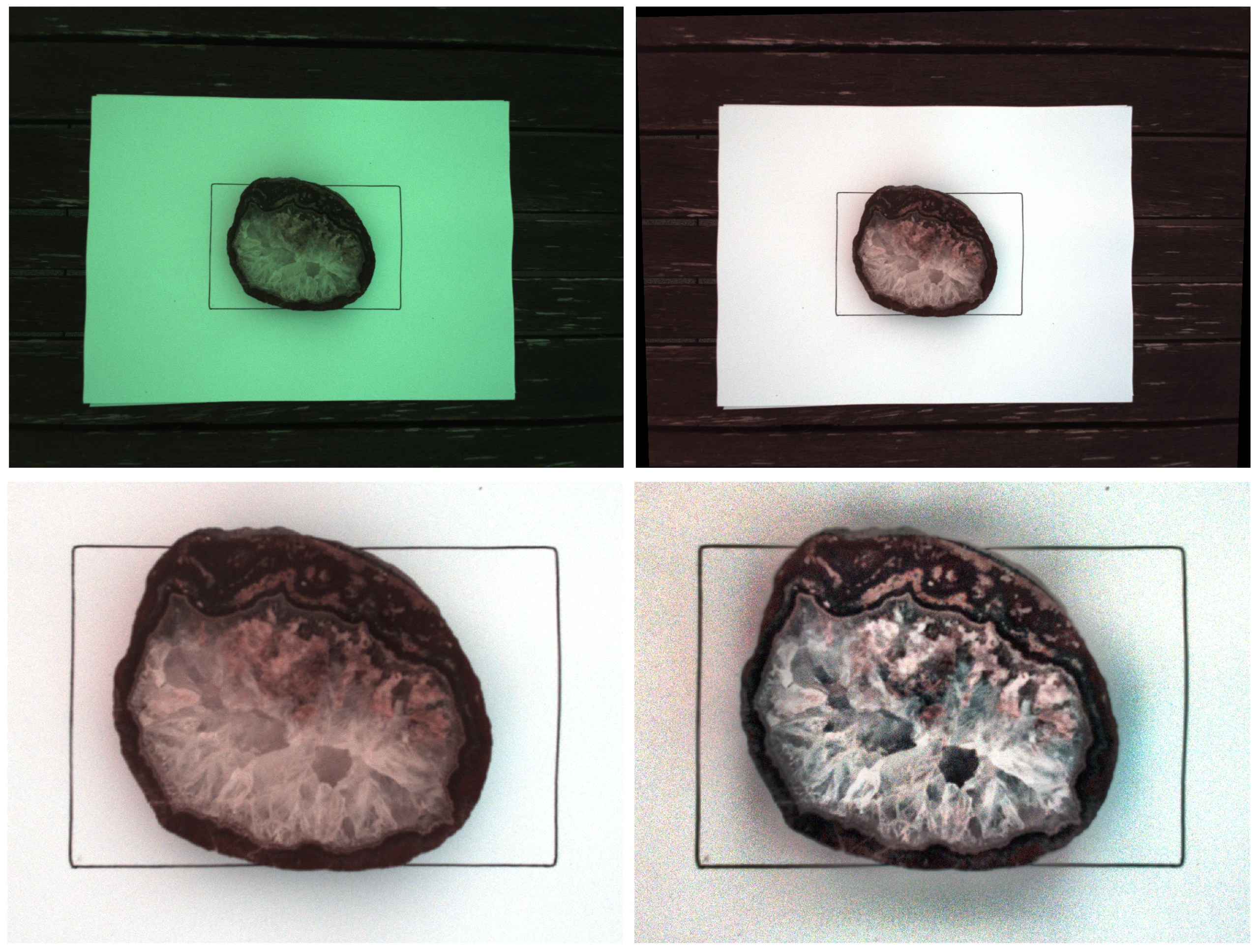
Finally, we can display the image before and after the white balance, before and after histogram equilization using
t = tiledlayout(2,2, ...
   'TileSpacing','compact');
nexttile, imshow(I3)
nexttile, imshow(I5)
nexttile, imshow(I6)
nexttile, imshow(I7)

print -dpng -r300 mapirsurvey3_615_490_808_1.png
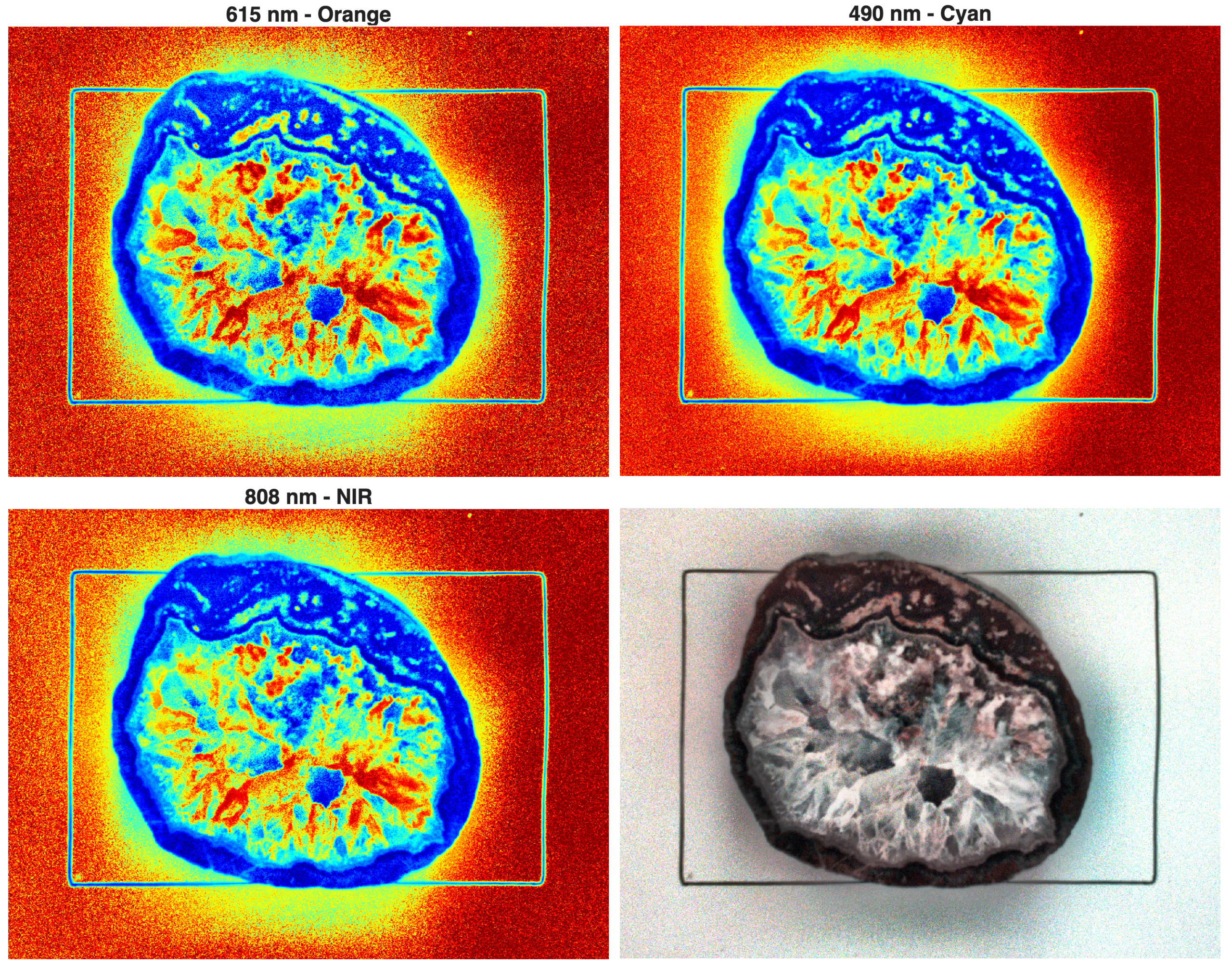
We can also display pseudocolor plots of the three channels orange, cyan and near infrared without adaptive histogram equalization:
cmap = 'jet';
t = tiledlayout(2,2, ...
   'TileSpacing','compact');
nexttile, imshow(I6(:,:,1))
title('615 nm - Orange'), colormap(cmap)
nexttile, imshow(I6(:,:,2))
title('490 nm - Cyan'), colormap(cmap)
nexttile, imshow(I6(:,:,3))
title('808 nm - NIR'), colormap(cmap)
nexttile, imshow(I6)

print -dpng -r300 mapirsurvey3_615_490_808_2.png
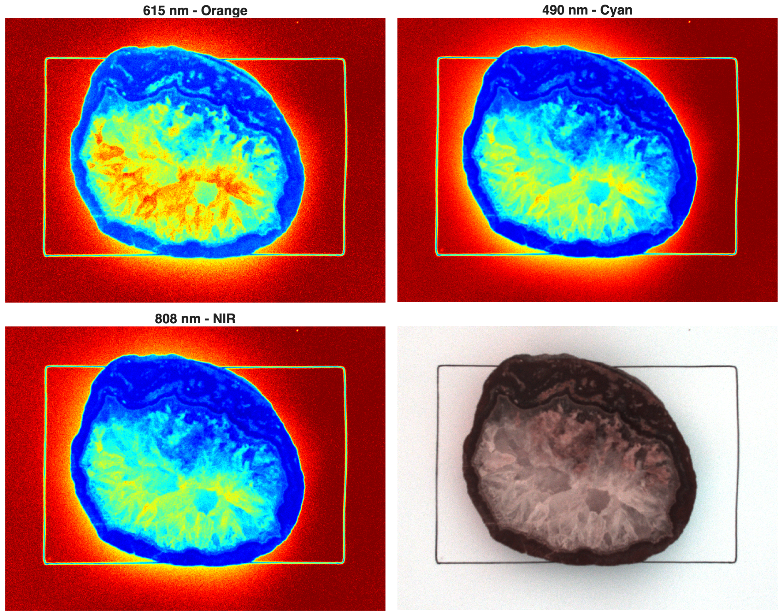
Alternatively, we can display pseudocolor plots of the three channels orange, cyan and near infrared after adaptive histogram equalization:
cmap = 'jet';
t = tiledlayout(2,2, ...
   'TileSpacing','compact');
nexttile, imshow(I7(:,:,1))
title('615 nm - Orange'), colormap(cmap)
nexttile, imshow(I7(:,:,2))
title('490 nm - Cyan'), colormap(cmap)
nexttile, imshow(I7(:,:,3))
title('808 nm - NIR'), colormap(cmap)
nexttile, imshow(I7)

print -dpng -r300 mapirsurvey3_615_490_808_3.png
In the last mosaic of images, you can clearly see that the red areas on the rock sample reflect more strongly in the orange wavelength range, while the quartz reflects more strongly in the cyan range, as expected.
References
Trauth, M.H. (2025) MATLAB Recipes for Earth Sciences – Sixth Edition. Springer International Publishing, 567 p.
Trauth, M.H. (2021) Signal and Noise in Geosciences, MATLAB Recipes for Data Acquisition in Earth Sciences. Springer International Publishing, 544 p.
Zuiderveld, K. (1994) Contrast Limited Adaptive Histograph Equalization. Graphic Gems IV. San Diego: Academic Press Professional, 474–485.