Importing and Displaying USGS Spectral Library Data with MATLAB

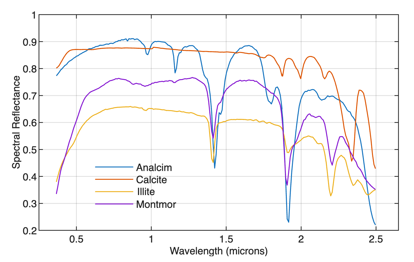
The USGS spectral library is an important database of mineral spectra, which is used as a reference for the spectrometric determination of unknown substances. Here is a simple MATLAB program that can be used to load and display the spectra of several minerals.

According to the USGS website, researchers at the USGS Spectroscopy Laboratory have measured the spectral reflectance of thousands of materials in the lab and compiled them in the USGS Spectral Library.  Detailed sample descriptions are provided with the spectra, including the results of X-ray Diffraction, Electron Probe Micro-Analysis, and other analytical methods.

First, we download the desired spectra from the USGS website:

https://www.usgs.gov/labs/spectroscopy-lab/usgs-spectral-library

We save the spectra and wavelengths in directories named spectraldata and wavelengths. We can then load this data using the following MATLAB commands to load the text files containing the wavelengths:

cd wavelengths
filelist_wv = dir(fullfile('*.txt'));
filename_wv = {filelist_wv.name};
for i = 1 : 1
   fidA = fopen(filename_wv{i});
   A1 = textscan(fidA,'%f',...
      'Headerlines',1,...
      'CollectOutput',1);
   fclose(fidA);
   wv(:,i) = A1{1};
end
cd ..

cd spectraldata
filelist_spec = dir(fullfile('*.txt'));
filename_spec = {filelist_spec.name};
for i = 1 : length(filelist_spec)
   fidB = fopen(filename_spec{i});
   B1 = textscan(fidB,'%f',...
      'Headerlines',1,...
      'CollectOutput',1);
   fclose(fidB);
   spec(:,i) = B1{1};
end
cd ..

for i = 1 : length(filelist_spec)
   legtex(i,:) = filename_spec{i}(10:14);
end

figure(...
   'Position',[200 200 800 600],...
   'Color',[1 1 1]);
axes(...
   'XLim',[0.25 2.65],...
   'Box','on',...
   'XGrid','On',...
   'YGrid','On',...
   'Units','Centimeters',...
   'Position',[2 2 10 6],...
   'LineWidth',0.6,...
   'FontName','Helvetica',...
   'FontSize',8);
for i = 1 : length(filelist_spec)
line(wv,spec(:,i),...
   'LineWidth',0.75)
end
xlabel('Wavelength (microns)',...
   'FontSize',8)
ylabel('Spectral Reflectance',...
   'FontSize',8)
legend(legtex,'Location','Southwest',...
   'FontSize',8)
legend('boxoff')

print -dpng -r300 usgs_spectrallibrary_2025.png

save usgs_spectrallibrary_2025.mat

Downloads

Download MATLAB script and data.

References

Trauth, M.H. (2025) MATLAB Recipes for Earth Sciences – Sixth Edition. Springer International Publishing, 550 p., ISBN 978-3-031-57948-6. (MRES)