
John Aitchison spent much of his career addressing the unique challenges of statistics for compositional data. His legacy is being carried on by colleagues who do not always succeed in presenting the material in a way that is understandable to geoscientists. Now in the fourth part of a series of blog posts, I am attempting to address the problems of closed data and possible workarounds using a series of simple MATLAB simulations, without frustrating geoscientists with mathematical formulas.
In fact, Pearson (1897) had already pointed out that spurious negative correlations occur in closed data: In a two-component system, one component increases to the same extent as the second component decreases. In my previous blog posts (Part 1, Part 2, and Part 3), I used a three-component system to show how two components, A and B, are diluted by a third component, C. These could be the allochthonous elements Fe and Ti in µXRF scans, which originate in marine sediments from terrestrial material input and are diluted by the autochthonous Ca, which originates from the CaCO3 shell-forming microorganisms.
In the literature, the Ca/Ti ratio is commonly used, in accordance with the recommendation by Aitchison (1999) and, due to the symmetry of the logarithm, often log(Ca/Ti). This is perfectly fine, but it is not a suitable measure for eliminating the diluting effect of Ca. On the contrary, it mixes the processes that control the input of Ti (e.g., the input of river sediments or dust) with the processes that control the amount of Ca (e.g., carbonate formation and preservation). Of course, dilution effects are indeed corrected, but not those one might expect: these are hidden influences on XRF measurements, such as fluctuating water content in the sediment, grain size effects, and a possible instrumental drift, the daily variation of the measuring device, which can also be determined by regularly measuring standards.
There is also a second problem, which Aitchison (1999) addressed. Ti usually accounts for two orders of magnitude smaller proportions of the total sediment and, due to its low content, has a much poorer signal-to-noise ratio than Ca. This can usually be seen very clearly in the fact that Ti, apart from the long-wave and counter-phase variations caused by dilution by Ca, shows a high-frequency fluctuation with large amplitude. This is the measurement error that superimposes white noise on the actual Ti content. If you divide Ca by Ti, you get nothing, but you lose much of the high signal-to-noise ratio of Ca. In the worst case, if the actual variation of Ti apart from dilution by Ca and white noise due to measurement errors is zero, a constant value is assigned without gaining anything.
Here is a simple MATLAB example illustrating the closed-sum problem of a system with three variables, and the use of ratios as well as log-ratios to overcome the problem of spurious correlations between pairs of variables. First, we clear the workspace and choose colors for the plots.
clear, close all, clc
colors = [
0 114 189
217 83 25
237 177 32
126 47 142
]./255;
We are interested in element 1a and element 1b, which are diluted by element 1c. We simply create three variables with magnitudes measured in milligrams, contributing to a sediment and with a sinusoidal variation of 200 samples down core. Make sure that all absolute values are >0.
t = 0.1 : 0.1 : 20; t = t';
element1a = sin(2*pi*t/2) + 5;
element1b = sin(2*pi*t/5) + 5;
element1c = 2*sin(2*pi*t/20) + 5;
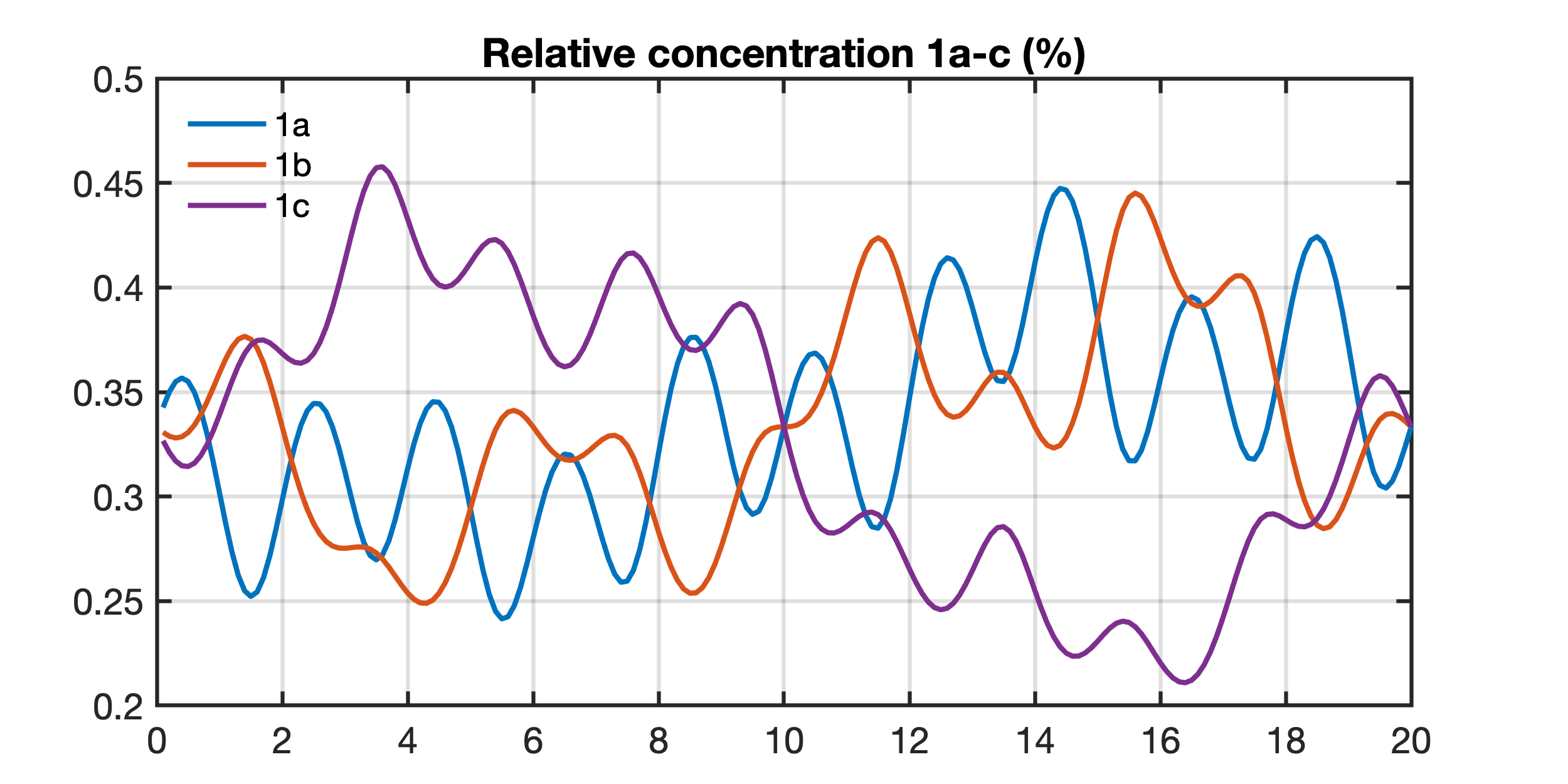
Calculating percentages of elements 1a-c, i.e. creating ratios of the individual elements and the sum of all elements. This process creates closed data, i.e. the data are now expressed as proportions and adding up to a fixed total of 100 percent, 1a+1b+1c = 100%. Now elements 1a and elements 1b are affected by the dilution by elements 1c. These elements show a significant sinusoidal long-term trend that is not real, as the first figure shows.
element1a_perc = element1a./...
  (element1a+element1b+element1c);
element1b_perc = element1b./...
  (element1a+element1b+element1c);
element1c_perc = element1c./...
  (element1a+element1b+element1c);

figure('Position',[100 700 600 300])
a2 = axes('Position',[0.1 0.1 0.8 0.8],...
  'Box','On',...
  'LineWidth',1.5,...
  'FontSize',14);
line(a2,t,element1a_perc,...
  'Color',colors(1,:),...
  'LineWidth',1.5);
line(a2,t,element1b_perc,...
  'Color',colors(2,:),...
  'LineWidth',1.5);
line(a2,t,element1c_perc,...
  'Color',colors(4,:),...
  'LineWidth',1.5);
legend('1a','1b','1c',...
  'Box','Off',...
  'Location','northwest'), grid
title('Relative concentration 1a-c (%)')
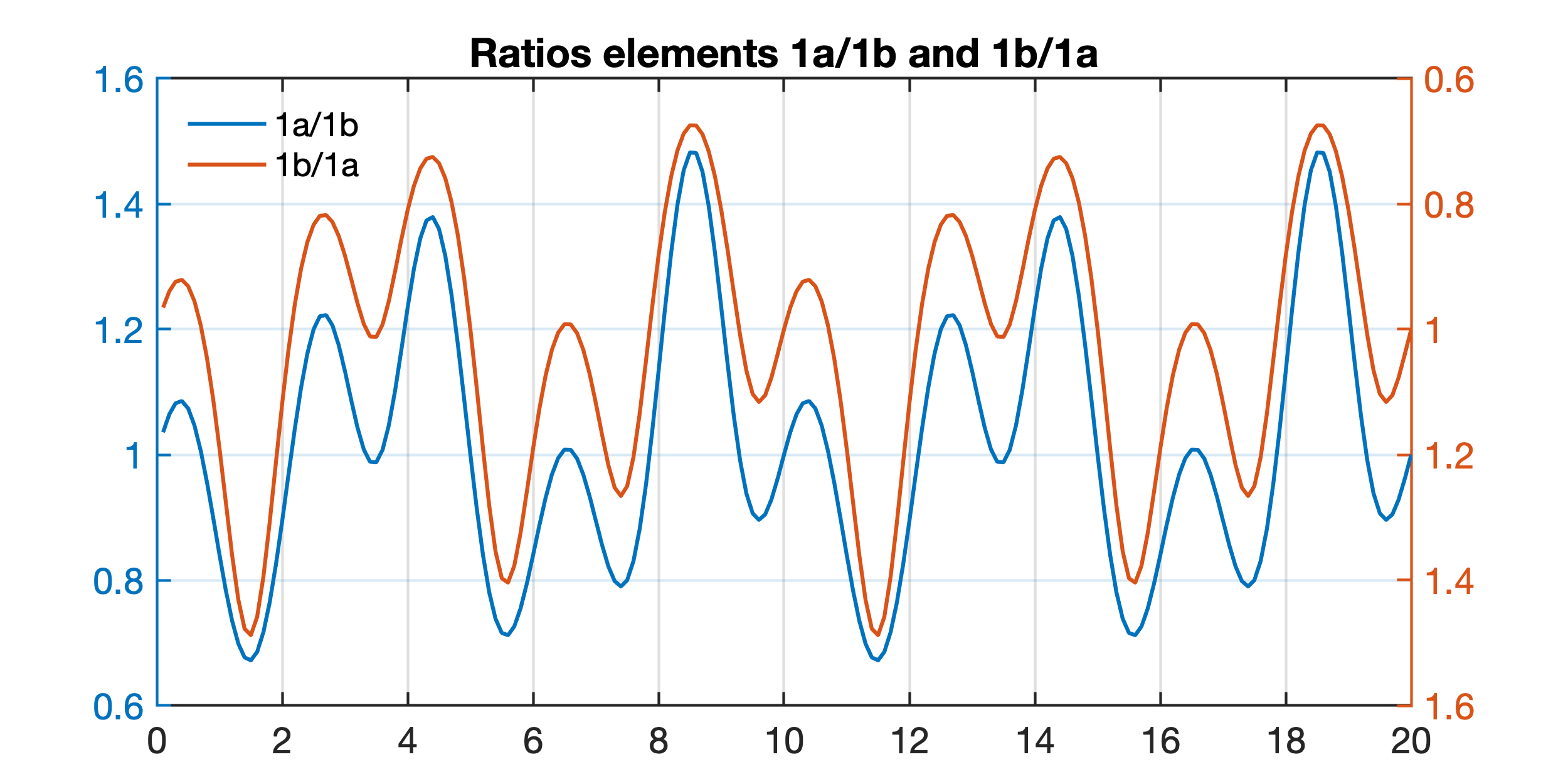
Built ratios of element 1a/1b and element 1b/1a, which are both independent from element 1c. Note the change of sign and difference in the amplitudes. The ratio of element 1a/1b and 1b/1a do not show the trend caused by the dilution effect of element 1c. However, the two curves are not identical, i.e. 1a/1b and 1b/1a are not symmetric (see Weltje and Tjallingii 2008, page 426).
ratio12 = element1a_perc./element1b_perc;
ratio21 = element1b_perc./element1a_perc;

figure('Position',[100 400 600 300])
a3 = axes('Position',[0.1 0.1 0.8 0.8],...
  'Box','On',...
  'LineWidth',1,...
  'FontSize',14);
yyaxis left, line(a3,t,ratio12,...
  'Color',colors(1,:),...
  'LineWidth',1.5);
yyaxis right, line(a3,t,ratio21,...
  'Color',colors(2,:),...
  'LineWidth',1.5);
set(a3,'YDir','Reverse')
legend('1a/1b',...
  '1b/1a',...
  'Box','Off',...
  'Location','northwest'), grid
title('Ratios elements 1a/1b and 1b/1a')
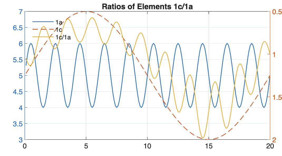
However, if we now form the ratio of element 1c/1a, i.e., Ca by Ti, we gain nothing: the diluting effect of element 1C remains is still there:
ratio31 = element1a_perc./element1c_perc;

figure('Position',[100 400 600 300])
axes('Box','On');
yyaxis left
line(t,element1a,...
  'Color',colors(1,:),...
  'LineWidth',1.5)
line(t,element1c,...
  'Color',colors(2,:),...
  'LineWidth',1.5)
yyaxis right
line(t,ratio31,...
  'Color',colors(3,:),...
  'LineWidth',1.5)
set(gca,'YDir','Reverse')
legend('1a',...
  '1c',...
  '1c/1a',...
  'Box','Off',...
  'Location','northwest'), grid
title('Ratios of Elements 1c/1a')
Again, maybe that i what interests you, but then you should not state in the methodology section of your paper that you want to use it to eliminate dilution effects in your data set. That won’t work that way. If element 1C is the diluting element that is negatively correlated with 1A and 1B, then you must divide 1A by 1B to eliminate the effect. Of course, if 1A and 1C are positively correlated, because they share the same process, then you lose a lot of the variance in these elements—but that’s just the way it is with closed data, which is why Aitchison has written so many papers and books on the subject.
References