Sustainable Code for GUI Tools / Apps with MATLAB

In 1994, as part of my doctorate, I programmed a graphical user interface for an adaptive filter using MATLAB. I have continued to develop the code over the past 30+ years. Here is the story of sustainable MATLAB code in four chapters.

Chapter 1

In the fall of 1992, I began a doctoral project at the University of Kiel in northern Germany on the deconvolution of bioturbated paleoceanographic time series. Earlier attempts to deconvolution bioturbation led to unrealistic fluctuations in the signal, which led to the false conclusion that bioturbation was overestimated. In fact, the noise in the paleoceanographic time series was amplified during deconvolution. Bioturbation acts as a low-pass filter, suppressing high-frequency signal components. However, if the signal is superimposed by high-frequency noise, both deconvolution and amplification occur.

The problem can be solved by suitable filtering of the time series prior to deconvolution. However, the arbitrary selection of filter parameters for noise suppression is unsatisfactory if a quantitative result is to be achieved in the deconvolution. The signal-to-noise ratio is not known for single measurements, but measuring a sample of ~150 foraminiferal shells is usually not feasible.

This is where adaptive filters can help, extracting a signal that is ~70% noise-reduced from double measurements. These filters were developed to better understand a pilot (signal s) in a noisy airplane (noise n) by setting up a second microphone elsewhere in the airplane (n only) to extract the noisefree s from s+n. I came across a paper by M. Hatting (1988), who presented a method for extracting a low-noise signal from double measurements s+n1 and s+n2, and I started to take an interest in adaptive filters.

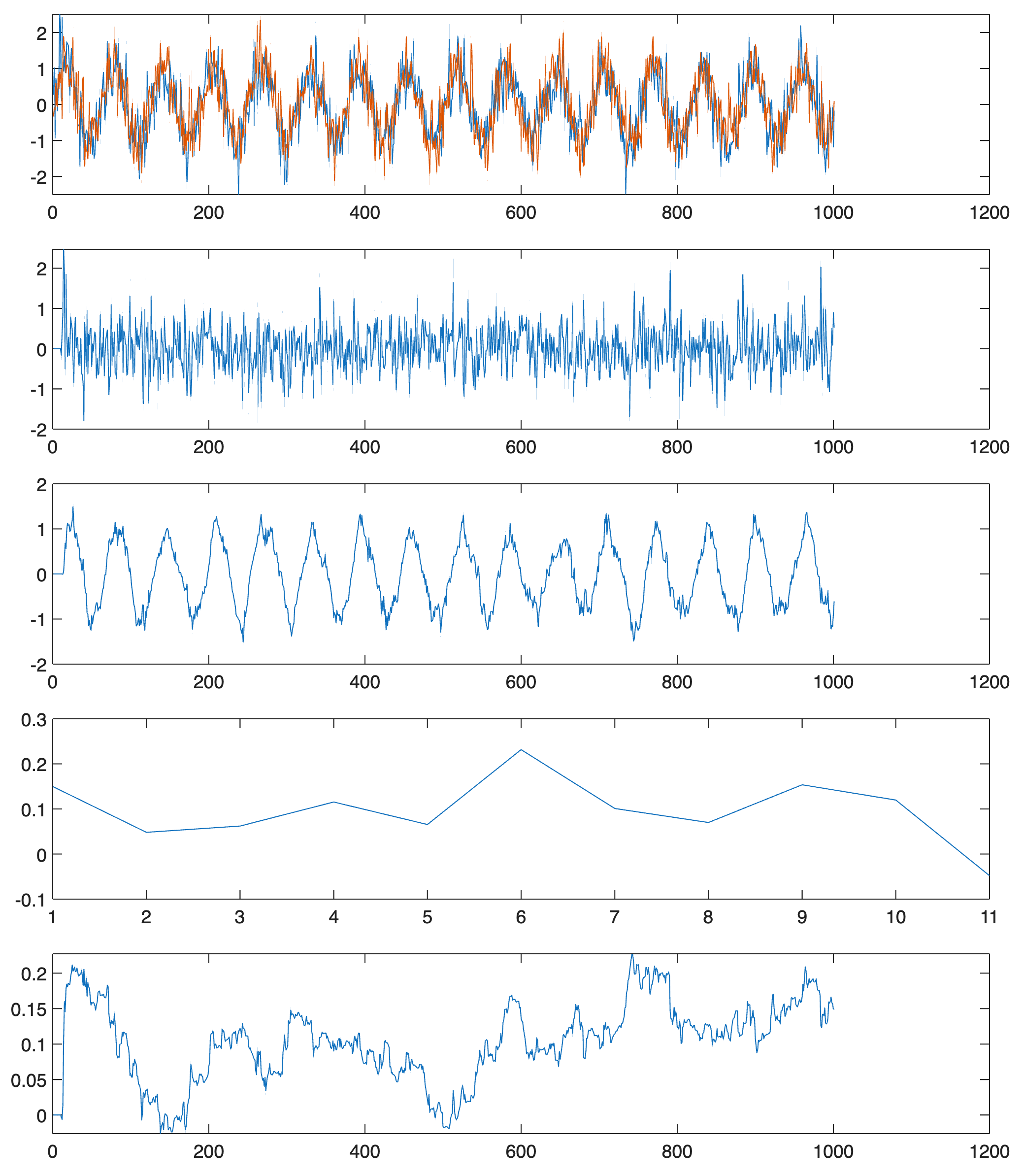
Looking for the MATLAB code, I searched a Usenet newsgroup and got in touch with Vijay Parsa at U Brunswick, now at Western U, who was filtering weak nerve signals with adaptive filters. He sent me his code for an LMS and an RLS filter, which inspired my own MATLAB codes. However, I had modified the filters in two ways: first, in the sense of Hatting for duplicate measurements. As an example, let us create a sine wave and then create to noisy versions of the signal yn1 and yn2 using

x = 0 : 0.1 : 100; x = x';
y = sin(x);
rng(0)
yn1 = y + 0.5*randn(size(y));
yn2 = y + 0.5*randn(size(y));

[error,fil_out,w1,wk] = lms2(yn1,yn2,11,0.01,5);

tiledlayout(5,1)
nexttile, plot(1:length(yn1),yn1,...
               1:length(yn2),yn2)
nexttile, plot(error)
nexttile, plot(fil_out)
nexttile, plot(w1)
nexttile, plot(wk)

I can’t remember exactly what inspired me back then to program the two LMS and RLS filters in a variant with a graphical user interface (GUI). Maybe it was one of the first examples that MathWorks presented back then. It was a simple GUI with a stylized thermometer in the middle with a red bar. To the left and right were text input fields where you could enter the temperature in degrees Celsius and Fahrenheit and thus convert it.

At that time, there were no tools for easy GUI programming, such as GUIDE and App Designer, so I used the code of the thermometer example as a template. Of course, this was very laborious compared to today, when the App Designer arranges interactive elements and axis systems as in a graphics program and automatically programs the associated code in the background.

Chapter 2

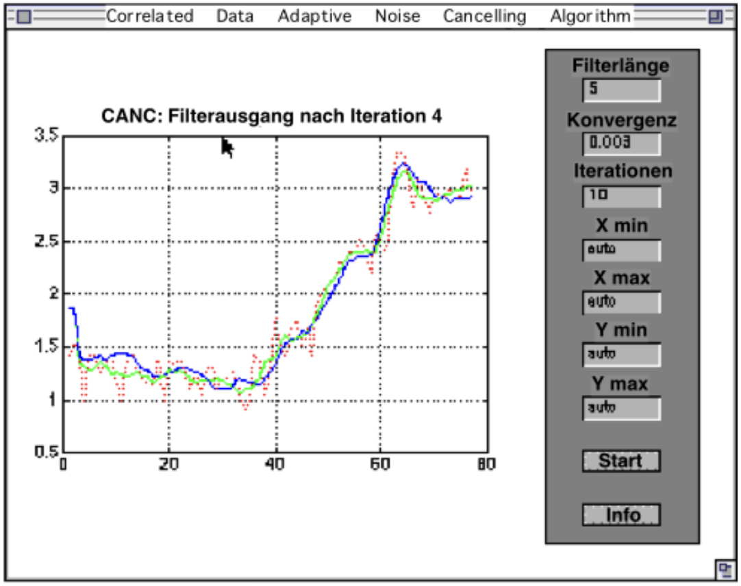
The 1994 code still works, but not without errors. However, I corrected all the errors a few years later; for example, save MER.m MER /ascii had to be replaced by save MER.m MER -ascii. This code in the file canc10.m still works without problems today, a GUI stored in a simple text file and programmed at the time with a lot of globals, which one would no longer do today. We can use the example data from above and start the GUI with the command

canc10(yn1,yn2)

A window with the GUI will open, where we can use the automatic values for the filter length, convergence factor, and number of iterations, or we can use our own values (see Trauth 2025 for details about adaptive filters). Unlike the original version, three line charts are displayed here, where in the original version the line charts were displayed one after the other in the window. However, the panel with the text input fields still looks very similar to the one in my dissertation.

Chapter 3

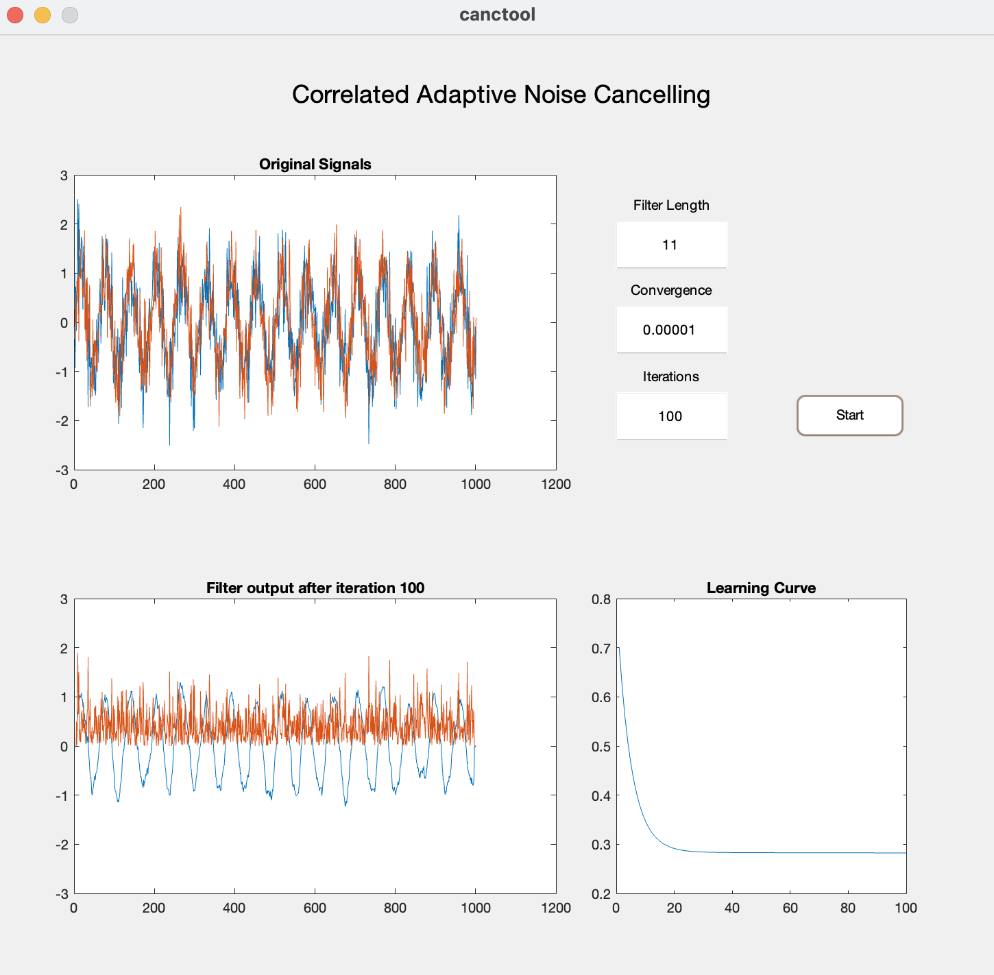
In the year 2000, the GUIDE (Graphical User Interface Development Environment) was introduced in MATLAB with version R12. GUIDE is a graphical user interface that makes it possible to create interactive GUIs (Graphical User Interfaces) without having to manually write a lot of code. I completely rewrote the adaptive filter with a graphical user interface using the GUIDE. The GUIDE generates two files, the actual MATLAB script with the filter canctool.m and the figure file canctool.fig. You can again use the above sample data and launch the filter using

canctool(yn1,yn2)

which yields the GUI with axes, text input fields and a start button. Again, you can keep the presets or you define your own values for the filter length, the convergence factor and the number of iterations, before you press the Start button. Similar to the previous version, you get four line charts with the input signals, the filter result and noise, and the learning curve.

Chapter 4

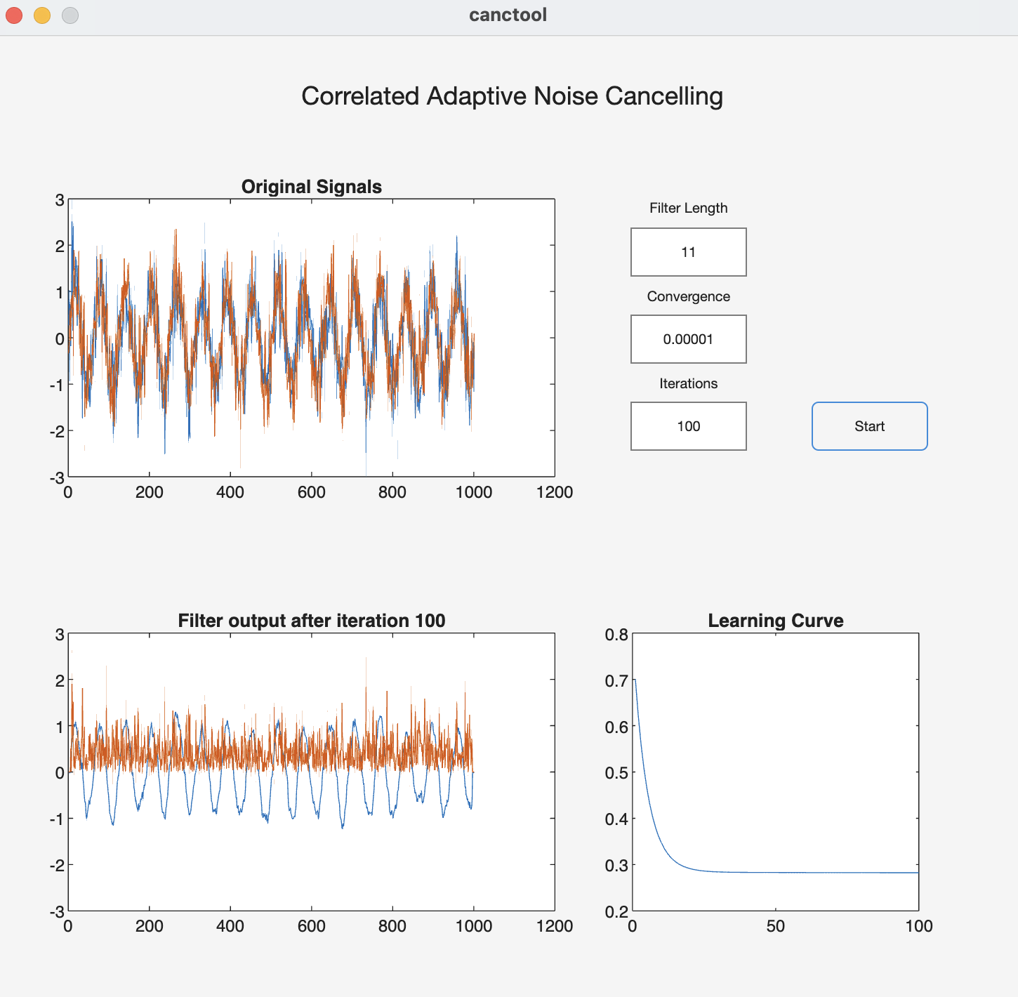
GUIDE was the main tool for GUI development in MATLAB until MATLAB R2018b, when it was replaced by App Designer. In fact, the GUIs created with the GUIDE could be used for a very long time, but now they are causing increasing difficulties. Thanks to the excellent MathWorks support, I was able to migrate the GUI created with the GUIDE without any problems. For this purpose, a guide on the MathWorks website describes how to use the appmigration.migrateGUIDEApp in release R2024b. It migrated the .m and .fig files from the GUIDE and converts them into the App Designer file canctool.mlapp. The result looks very similar to the GUI from the GUIDE and can be started again with the command

canctool(yn1,yn2)

which yields the GUI with axes, text input fields and a start button. Again, you can keep the presets or you define your own values for the filter length, the convergence factor and the number of iterations, before you press the Start button. Similar to the previous version, you get four line charts with the input signals, the filter result and noise, and the learning curve.

As you can see, it is certainly possible to migrate older GUIs, but can you be sure that it will work for another 30 years? The code from 1994 no longer works without difficulties, but the code from 1994 does work – but for how much longer? That’s why it’s always important to store data and code in a format, e.g. a classic script in an ASCII or UTF-8 text file, that will probably still work, like the early versions of the filter from 1994. And if at some point there is no interpreter for the MATLAB language, you can probably still understand the code because the language is a mathematical language. The App Designer  .mlapp cannot be read with a text editor, but it can export as .m files, which can be very useful.

References

Hattingh, M. (1988) A new data adaptive filtering program to remove noise from geophysical time- or space series data: Computers & Geosciences, 14, 467-480.
Trauth, M. H. (1995) Bioturbate Signalverzerrung hochaufloesender palaeoozeanographischer Zeitreihen: Berichte—Reports, Geologisch-Palaontologisches Institut der Universitat Kiel, v. 74, 167 p.
Trauth, M.H. (1998) Noise removal from duplicate paleoceanographic time-series: The use of adaptive filtering techniques. Mathematical Geology, 30(5), 557-574.
Trauth, M.H. (2025) MATLAB Recipes for Earth Sciences – Sixth Edition. Springer International Publishing, 567 p, https://doi.org/10.1007/978-3-031-57949-3.
Widrow, B., Hoff, M., Jr. (1960) Adaptive switching circuits: IRE WESCON Conv. Rev., 4, 96-104.