
Artificial neural networks (ANNs) have been used for quite some time to identify, for example, flowers in easy-to-use apps on smartphones. They have been, however, the focus of great attention since the introduction of generative artificial intelligence chatbots like OpenAI’s ChatGPT.
Introduction
There are numerous convenient tools in MATLAB and the Deep Learning Toolbox (MathWorks 2025b) that make it easy to get started with ANNs, but the examples used in the documentation, tutorials and are usually very complex. For an easy introduction to the topic of machine learning in general and ANNs in particular, the excellent videos on Grant Sanderson’s 3Bue1Brown YouTube channel, which have become very popular (Sanderson 2017). On his website and YouTube Channel you will find a section about ANNs in general including the introduction But what is a Neural Network?. There is nothing comparable on the web so far that explains complex topics in maths and computer science with such simple, yet skilfully crafted animations.
The following simple MATLAB example shows an ANN with backpropagation, inspired by a Python script, which can be found in numerous variants on the internet, but probably originally goes back to a blog post by Trask (2015). Another inspiration is the article on ANNs on the German Wikipedia (12 February 2025), whose naming of the variables we have also adopted.
Step 1 – Designing the Artificial Neural Network
We first clear the workspace by typing
clear, close all, clc
Then, we define a learning rate or step size alp to improve the weights w. As always with such iterative learning algorithms, the rate is a compromise between fast learning and accurate learning. You can play around with different values for alp and see the difference in the graphics below:
alp = 0.1;
Our training data set consists of four samples of three values each, such as four different samples of climate transitions characterized by three parameters, such as the mean, the standard deviation, and the skewness of some climate variable. We therefore create a very simple ANN with an input layer x with three input nodes (e.g. three artificial neurons) corresponding to the three parameters:
x = [0 0 1
     1 1 1
     1 0 1
     0 1 1];
The output layer of the ANN contains the expected output of the training data set, that is, the Type 0 or 1 of the respective climate transition of the four samples in the training data set. As you can see, the first and last sample should be characterized by Type 0 of climate transition and the second and third sample should be of Type 1. We have only one column and therefore only one output node:
y = [0
     1
     1
     0];
The ANN essentially consists of the array of weights w, which are iteratively improved in the course of training the network. In our example, we only have one set of three weights w because we only have one input layer x and one output layer y, which are linked by the weights w. We use random values for the initial weights w, where the sum of the weights is one.
rng(0)
w = rand(3,1);
w = w/sum(w)
Step 2 – Training the Artificial Neural Network
We train the network iteratively in which the best values for the weights w are to be found in order to find oj as a prediction of the output y. The training is realized by a for loop:
for i = 1 : 100
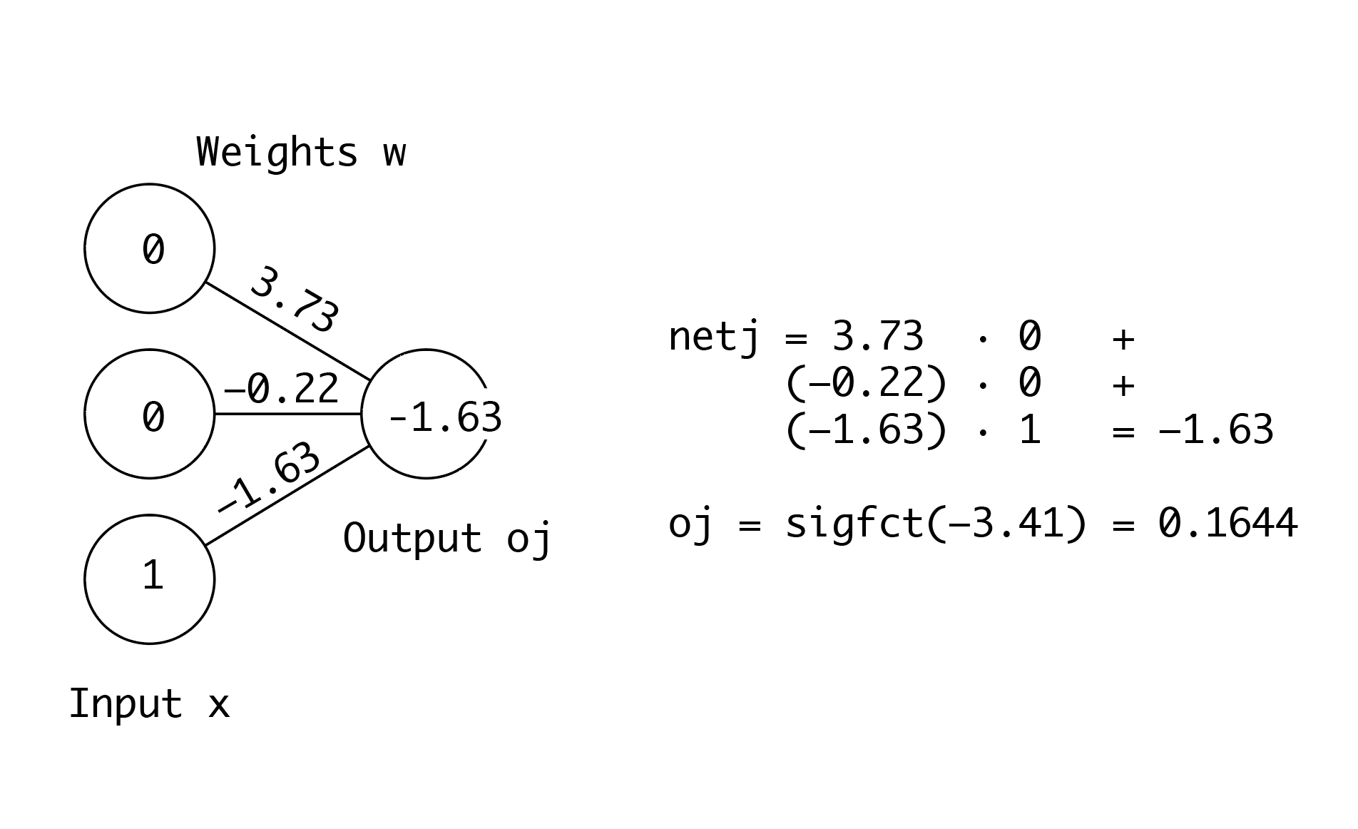
When the neuron receives the input x it first computes a propagation function netj, which usually is the sum of the input x weighted by w or, in other words, the inner product of x and w.
netj = x*w;
After the propagation function netj, the activation function is applied, which brings the nonlinearity into the network, to compute an estimate of the output oj. There are many different functions used as activation function. The rectifier function or rectified linear unit (ReLU) is often used in the hidden layers (not used here), while the sigmoid function sigfct (see below) is used in the output layer:
oj = sigfct(netj);
The code for the sigmoidal function as an example of an activation function sigfct can be found below, outside the for loop (Step 6). The filter weights w are found using error backpropagation. To do this, we first calculate the gradients of the error function as a function of the weights, in our case this is the derivative of the sigmoid function sigfctderiv. The weights are then updated on the basis of the gradients using a steepest descent approach with the stepsize alp.
w = w + alp*x'*(sigfctderiv(netj).*(y-oj));
Again, the code for the activation function’s derivative sigfctderiv can be found below, outside the for loop (Step 6). We store the values for the mean squared error E, the prediction of the output oj and the weights w for each i of the for loop in order to graphically represent the iterative learning of the network below:
   Ei(:,i) = E;
   oji(:,i) = oj;
   wi(:,i) = w;
At the end, we need an end to close the for loop to train the network iteratively:
end
In our example, after 100 passes through the for loop, we have now successfully trained our ANN. In the next steps, we will look at the quality of the prediction of the known output y and then use the network for a prediction of an unknown sample.
Step 3 – Evaluating the ANN Training Results
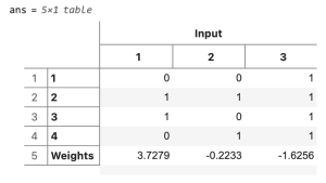
We now have a fully trained ANN whose input values and weights we can clearly display in a table by typing
table(cat(1,x,w'),...
   'VariableNames',["Input"],...
   'RowNames',["1","2","3","4","Weights"])
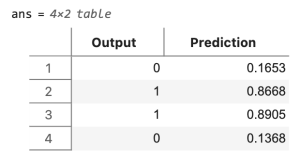
You can see that the predicted value oj of the output y is very good, as you can see by typing
table(y,oj,...
'VariableNames',["Output","Prediction"])
Step 4 – Prediction
You can now use the trained ANN for prediction, e.g. to determine the Type 0 or 1 of any sample, such as
s = [0 0 1];
sigfct(s*w)

ans = 0.0319
As you can see, you get the expected result of a value close to zero.
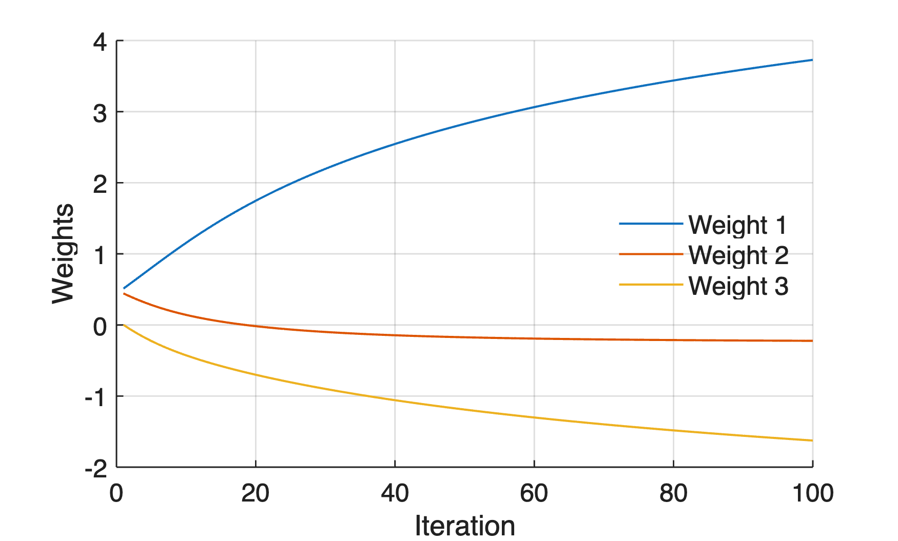
Step 5 – Graphical Display of the ANN Training
We can now graphically display the weights w during the training by typing:
axes('LineWidth',0.7,...
   'FontSize',12,...
   'XGrid','On',...
   'YGrid','On')
line(1:length(wi),wi,...
   'LineWidth',1)
xlabel('Iteration')
ylabel('Weights')
legend('Weight 1','Weight 2','Weight 3',...
   'FontSize',12,...
   'Location','East',...
   'Box','Off')

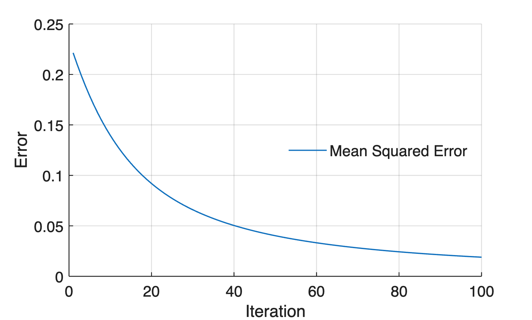
Accordingly, we can also graphical display of the mean squared error E during the training of the ANN:
figure
axes('LineWidth',0.7,...
   'FontSize',12,...
   'XGrid','On',...
   'YGrid','On')
line(1:length(Ei),Ei,...
   'LineWidth',1)
xlabel('Iteration')
ylabel('Error')
legend('Mean Squared Error',...
   'FontSize',12,...
   'Location','East',...
   'Box','Off')

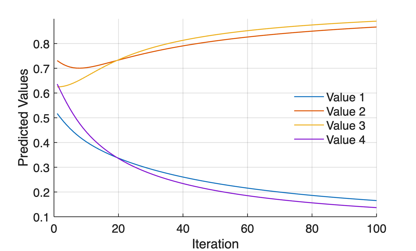
Accordingly, we can also graphical display of the predicted value oj of the output y during the training:
figure
axes('LineWidth',0.7,...
   'FontSize',12,...
   'XGrid','On',...
   'YGrid','On')
line(1:length(oji),oji,...
   'LineWidth',1)
xlabel('Iteration')
ylabel('Predicted Values')
legend('Value 1','Value 2','Value 3','Value 4',...
   'FontSize',12,...
   'Location','East',...
   'Box','Off')
Step 6 – The Activation Function
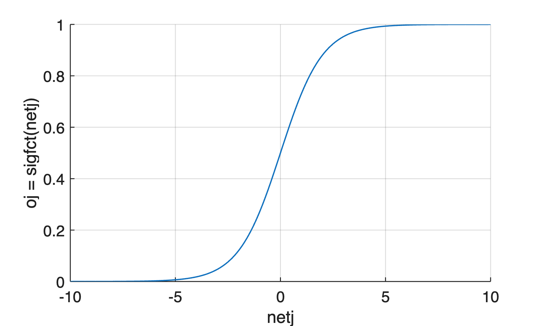
In this 6th step, the activation function and its derivation for the optimization of the weights as well as their graphical representation are compiled. First, we look at the sigmoid function sigfct as an activation function. Please note that the input argument x and output argument y of the function used here are not identical to the input and output x and y in the ANN example. We type
function y = sigfct(x)
   y = 1./(1+exp(-x));
end
We use the following code to graphically display of sigmoid function:
xx = -10 : 0.1 : 10;
yy = sigfct(xx);

figure
axes('LineWidth',0.7,...
   'FontSize',12,...
   'XGrid','On',...
   'YGrid','On')
line(xx,yy,...
   'LineWidth',1)
xlabel('netj')
ylabel('oj = sigfct(netj)')
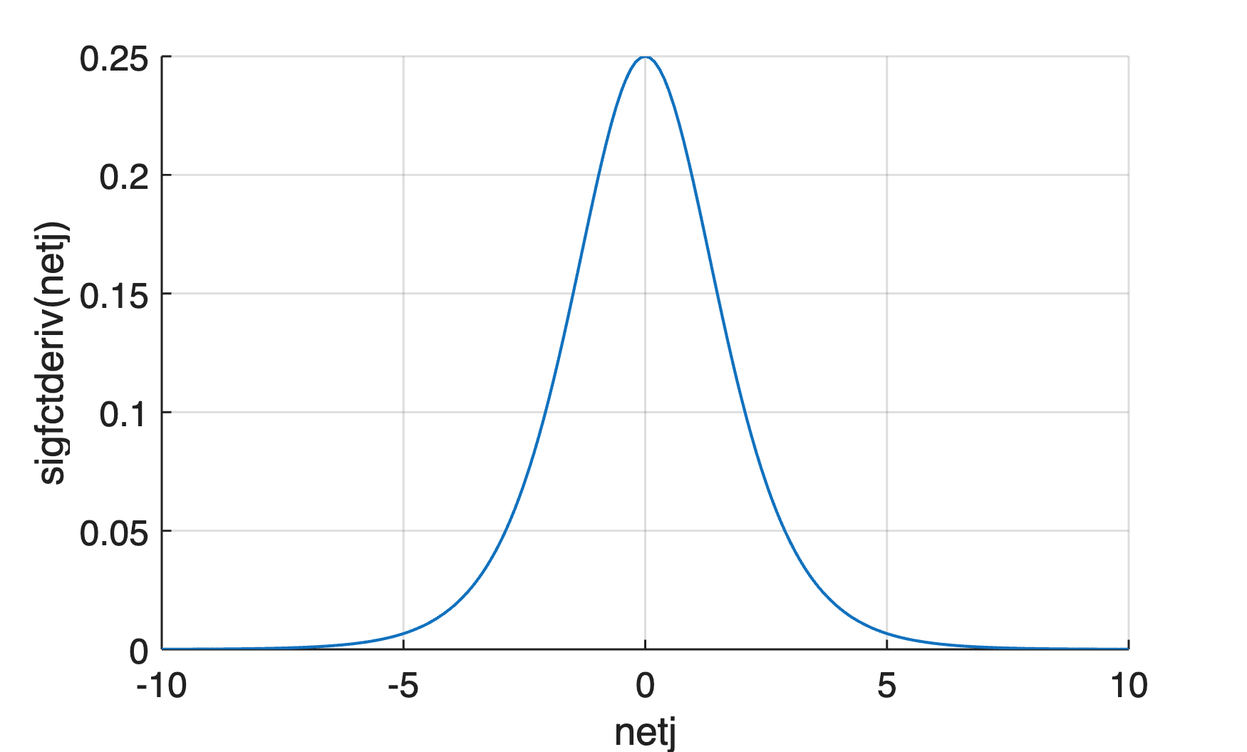
We use the function sigfctderiv to calculate the derivative of the sigmoid function:
function y = sigfctderiv(x)
y = sigfct(x).*(1 - sigfct(x));
end
We use the following code to graphically display the derivative of sigmoid function:
xx = -10 : 0.1 : 10;
yy = sigfctderiv(xx);

figure
axes('LineWidth',0.7,...
   'FontSize',12,...
   'XGrid','On',...
   'YGrid','On')
line(xx,yy,...
   'LineWidth',1)
xlabel('netj')
ylabel('sigfctderiv(netj)')
References
Trask, A. (2015) A neural network in 11 lines of Python (Part 1), I am Trask, A Machine Learning Craftsmanship Blog (Link).
Sanderson, G. (2017) Neural networks – The basics of neural networks, and the math behind how they learn (Link).
Daniel Sonnet (2022) Neuronale Netze kompakt, Vom Perceptron zum Deep Learning. Springer Vieweg, Berlin.