Color is an uncertain characteristic for the determination of minerals. Many minerals occur in a variety of different colors. Examples are quartz with its color variants amethyst, rose quartz or smoky quartz or feldspar with color variants like amazonite. However, if the minerals in a rock are reliably determined, their different coloring can be used to quantify them.
In the next example we use a simple RGB photo taken with a smartphone to determine the amounts of quartz, plagioclase, alkali feldspar and dark minerals such as biotite and hornblende in granite. To facilitate the differentiation of minerals, we use a principal component analysis (PCA), which is also used to unmix and classify spectral images such as satellite images (Trauth, 2020).
Exercise
- Use the smartphone RGB camera to acquire an image of a surface plate of granite. Make sure that the image is evenly illuminated.
- Use a principal component analysis to classify the minerals quartz, plagioclase, alkali feldspar alongside dark minerals such as biotite and hornblende.
- Use thresholds to separate the mineral content. Determine the relative proportions of minerals based on the number of pixels in the classified image. Display the result graphically in the form of mineral maps.
Solution
- Switch on the camera and take a picture of the granite surface plate. Make sure that the image is evenly illuminated.
- Use MATLAB script to import images and run the principal component analysis.
- Define thresholds to separate the minerals and count the pixels. Display the result.
MATLAB Script
We first define a file name and read the data from the visible light RGB (~370–650 nm) camera in a uint8 array in MATLAB.
clear, close all, clc
I1 = imread('IMG_2666.jpeg');
We then adjust the colors of the image using
I1(:,:,1) = imadjust(I1(:,:,1));
I1(:,:,2) = imadjust(I1(:,:,2));
I1(:,:,3) = imadjust(I1(:,:,3));
We then reshape 3,024-by-4,032-by-3 array of the image into a 12,192,768-by-3 array, i.e. the 12,192,768 pixels are the rows of the array and the three colors Red, Green and Blue are the columns.
I2 = reshape(I1,[size(I1,1)*size(I1,2) size(I1,3)]);
We convert the uint8 to a double array using a principal component analysis (PCA). Principal component analysis (PCA) detects linear dependencies between p variables and replaces groups of linearly correlated variables with p uncorrelated variables, referred to as the principal components (PCs) (Pearson, 1901, Hotelling 1931, Trauth, 2020). PCA is commonly used to unmix (or separate or decorrelate) the variables, which are a linear combination of independent source variables, the PCs.
I2 = double(I2);
[coeff,newdata,~,~,variance] = pca(I2);
The decorrelated variables are stored in newdata, converted back to the original dimensions of the image and store the result in I3.
I3 = reshape(newdata,size(I1));
We then display the original image together with the three principal component scores I3(:,1), I3(:,2) and I3(:,3) in separate images using imagesc.
figure('Position',[100 200 800 600])
axes('Position',[0.05 0.55 0.4 0.4])
imagesc(I1), axis off
title('RGB'), colorbar
axes('Position',[0.50 0.55 0.4 0.4])
imagesc(I3(:,:,1)), axis off
title('PC1'), colorbar
axes('Position',[0.05 0.10 0.4 0.4])
imagesc(I3(:,:,2)), axis off
title('PC2'), colorbar
axes('Position',[0.50 0.10 0.4 0.4])
imagesc(I3(:,:,3)), axis off
title('PC3'), colorbar
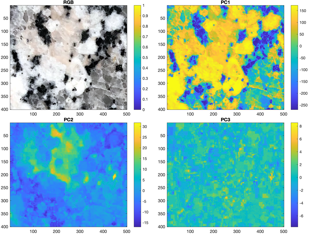
We can also zoom into a small area of the image to better see the individual minerals.
figure('Position',[100 1000 800 600])
axes('Position',[0.05 0.55 0.4 0.4])
imagesc(I1(800:1200,1000:1500,:))
title('RGB'), colorbar
axes('Position',[0.50 0.55 0.4 0.4])
imagesc(I3(800:1200,1000:1500,1))
title('PC1'), colorbar
axes('Position',[0.05 0.10 0.4 0.4])
imagesc(I3(800:1200,1000:1500,2))
title('PC2'), colorbar
axes('Position',[0.50 0.10 0.4 0.4])
imagesc(I3(800:1200,1000:1500,3))
title('PC3'), colorbar
We then binarize the three principal component scores using individual thresholds -50, 5 and 50. The threshold values are determined interactively by trial-and-error in order to achieve an optimal result.
I3T(:,:,1) = imbinarize(I3(:,:,1),-50);
I3T(:,:,2) = imbinarize(I3(:,:,2),5);
I3T(:,:,3) = imbinarize(I3(:,:,1),50);
We then create masks of zeros to hide areas where the individual minerals are not present.
I4_M = zeros(size(I3T(:,:,1)));
I4_M(I3T(:,:,1)==0) = 1;
I4_K = zeros(size(I3T(:,:,1)));
I4_K(I3T(:,:,2)==1) = 1;
I4_P = zeros(size(I3T(:,:,1)));
I4_P(I3T(:,:,3)==1 & I3T(:,:,2)==0) = 1;
I4_Q = zeros(size(I3T(:,:,1)));
I4_Q(I3T(:,:,1)==1 & I4_K==0 & I4_P==0) = 1;
We then create a new array I4 to store all four minerals.
I4(:,:,1) = I4_M;
I4(:,:,2) = I4_K;
I4(:,:,3) = I4_P;
I4(:,:,4) = I4_Q;
Finally, we present the result by creating four images for the individual minerals biotite+hornblende, alkali feldspar, plagioclase and quartz, where the minerals are shown in black and areas without the minerals are white (Fig. 6.exercise_6.6.3_1).
figure('Position',[100 100 800 600])
axes('Position',[0.05 0.55 0.4 0.4])
imagesc(I4(800:1200,1000:1500,1))
title('Biotite and Hornblende'), colorbar
axes('Position',[0.50 0.55 0.4 0.4])
imagesc(I4(800:1200,1000:1500,2))
title('Potassium Feldspar'), colorbar
axes('Position',[0.05 0.10 0.4 0.4])
imagesc(I4(800:1200,1000:1500,3))
title('Plagioclase'), colorbar
axes('Position',[0.50 0.10 0.4 0.4])
imagesc(I4(800:1200,1000:1500,4))
title('Quartz'), colorbar
Counting the pixels of individual minerals and dividing by the total number of pixels gives the percentage of minerals in the image
Total_Pixels = size(I1(:,:,1),1) * size(I1(:,:,1),2);
Total_M = 100*sum(sum(I4(:,:,1)==1))/Total_Pixels
Total_K = 100*sum(sum(I4(:,:,2)==1))/Total_Pixels
Total_P = 100*sum(sum(I4(:,:,3)==1))/Total_Pixels
Total_Q = 100*sum(sum(I4(:,:,4)==1))/Total_Pixels
which yields
Total_M = 31.2349
Total_A = 17.9549
Total_P = 33.7585
Total_Q = 19.6854
As we can see we have ~31% biotite+hornblende (M, which stands for mafic), ~18% alkali feldspar (A), ~34% plagioclase and ~20% quartz. We can save the data in a .mat file. The exercise demonstrates the complete workflow of a classification of minerals with the help of a PCA, as it is done in remote sensing.
Download the MATLAB script and example image.

