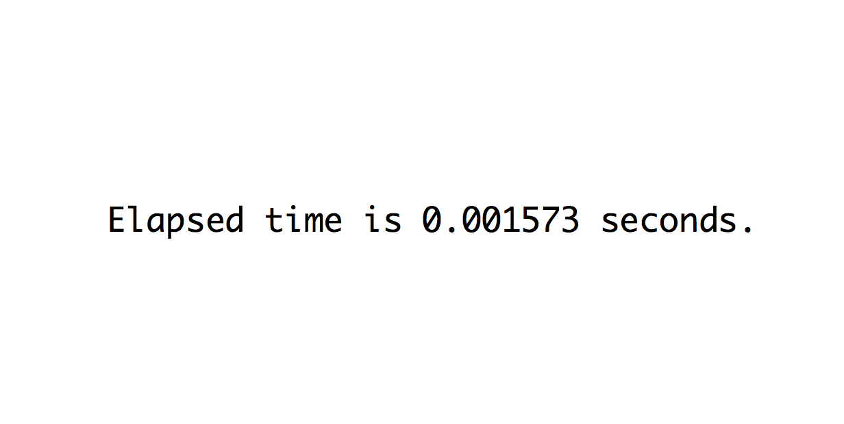
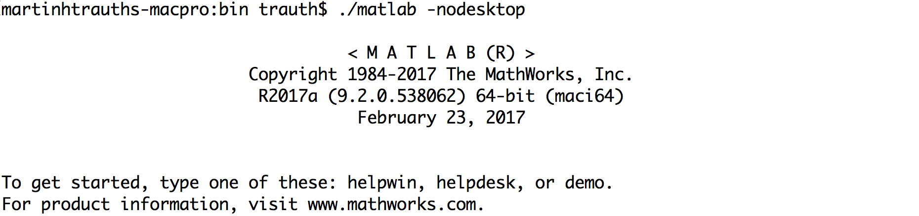
Principal Component Analysis in 6 Steps

The Principal Component Analysis (PCA) is equivalent to fitting an n-dimensional ellipsoid to the data, where the eigenvectors of the covariance matrix of the data set are the axes of the ellipsoid. The eigenvalues represent the distribution of the variance among each of the eigenvectors. To understand the method, it is helpful to know something about matrix algebra, eigenvectors, and eigenvalues. Here is a n=2 dimensional example to perform a PCA without the use of the MATLAB function pca, but with the function of eig for the calculation of eigenvectors and eigenvalues. Continue reading “Principal Component Analysis in 6 Steps”

Public Lecture on Climate Change and Human Evolution at U Potsdam Children’s University

On September 29, 2017, the University of Potsdam will once again open its lecture halls for children to inspire them with the world of science. On this day, children can listen to interesting lectures, discuss with the scientists, and can experience exciting experiments. On Friday 29 September 2017 I will give a public lecture on tectonics, climate and human evolution for 8–10 year old children. Please visit the webpage of the children’s university to learn more about the event and how to register.

Data Voids and Spectral Analysis: Don’t Be Afraid Of Gaps!

During a workshop on time series analysis on paleoclimatic data, I was asked how data gaps affect the results of spectral analyzes. The good news is, the expected climatic cycles such as Milankovitch cycles do not shift when the time series has gaps. However, it is important that the data is properly pre-treated before being examined with a method of spectral analysis. Continue reading “Data Voids and Spectral Analysis: Don’t Be Afraid Of Gaps!”

Using a Multispectral Array with MATLAB, Part 2

Using the MAPIR Survey2 cameras described in an earlier post I took photos of the car park next to our departmental building. The relatively inexpensive multispectral array consists of four cameras, ~340 € each, recording NDVI Red+NIR (650 and 850 nm), Blue (450 nm), Green (550 nm) and Visible Light RGB (~370–650 nm). We use the four cameras to build a multispectral array, possibly mounted on drones, to determine various types of minerals, vegetation, and man-made materials on the ground.

Continue reading “Using a Multispectral Array with MATLAB, Part 2”