
Quantifying the composition of substances in geosciences, such as the mineral composition of a rock in thin sections, or the amount of charcoal in sieved sediment samples, is facilitated by the use of image processing methods. Thresholding provides a simple solution to segmenting objects within an image that have different coloration or grayscale values. As an example we use thresholding to separate the dark charcoal particles and count the pixels of these particles after segmentation.
Quantifying the composition of substances in earth sciences (e.g., the mineral composition of a rock in thin sections or the amount of charcoal in sieved sediment samples) is facilitated by the use of image processing methods. Thresholding provides a simple solution to problems associated with segmenting objects within an image that have different coloration or grayscale values. During the thresholding process, pixels with an intensity value greater than a threshold value are marked as object pixels (e.g., pixels that represent charcoal in an image), and the rest are marked as background pixels (e.g., all other substances). The threshold value is usually defined manually by visually inspecting the image histogram, but numerous automated algorithms are also available.
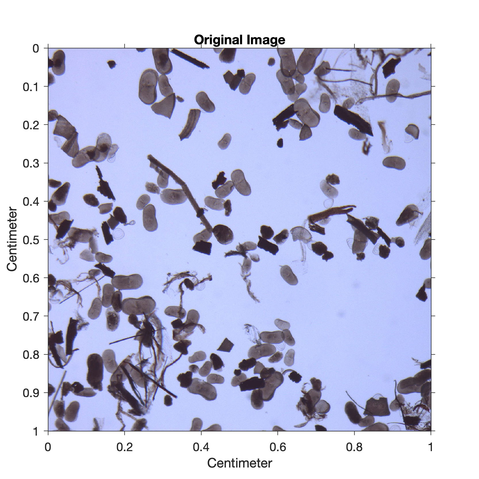
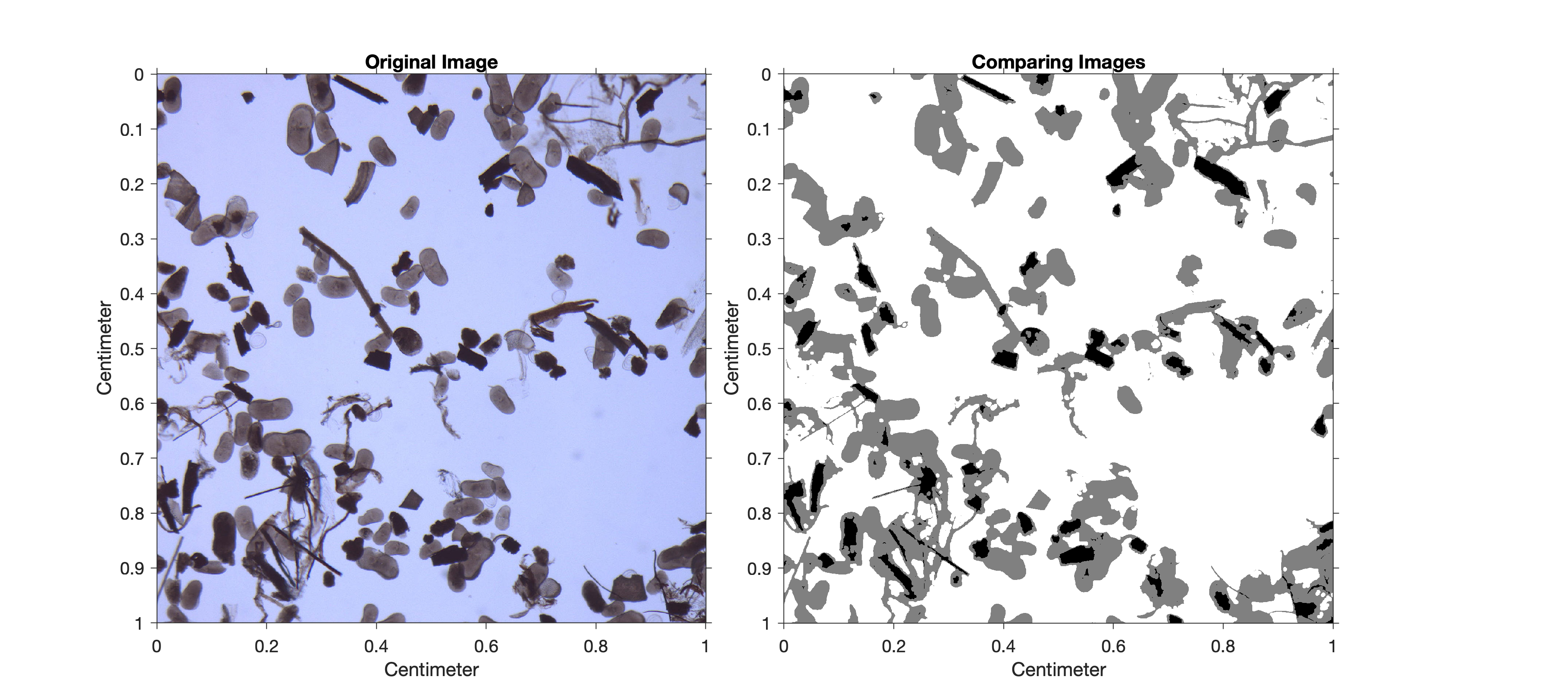
As an example, we next analyze an image of a sieved lake sediment sample from Lake Nakuru, Kenya (Fig. 8.10). The image shows abundant light-gray oval ostracod shells and some mineral grains as well as gray plant remains and black charcoal fragments. We use thresholding to separate the dark charcoal particles and count the pixels of these particles after segmentation. After determining the number of pixels for all objects that can be distinguished from the background by thresholding, we use a lower threshold value to determine the ratio of the number of pixels that represent charcoal to the number of pixels that represent all particles in the sample (i.e., to determine the percentage of charcoal in the sample).
We read the image of size 1,500-by-1,500 pixels and assume that the width and height of the square image are both one centimeter:
I1 = imread('lakesediment.jpg');
ix = 1; iy = 1;

imshow(I1,...
   'XData',[0 ix],...
   'YData',[0 iy]), axis on
xlabel('Centimeter')
ylabel('Centimeter')
title('Original Image')
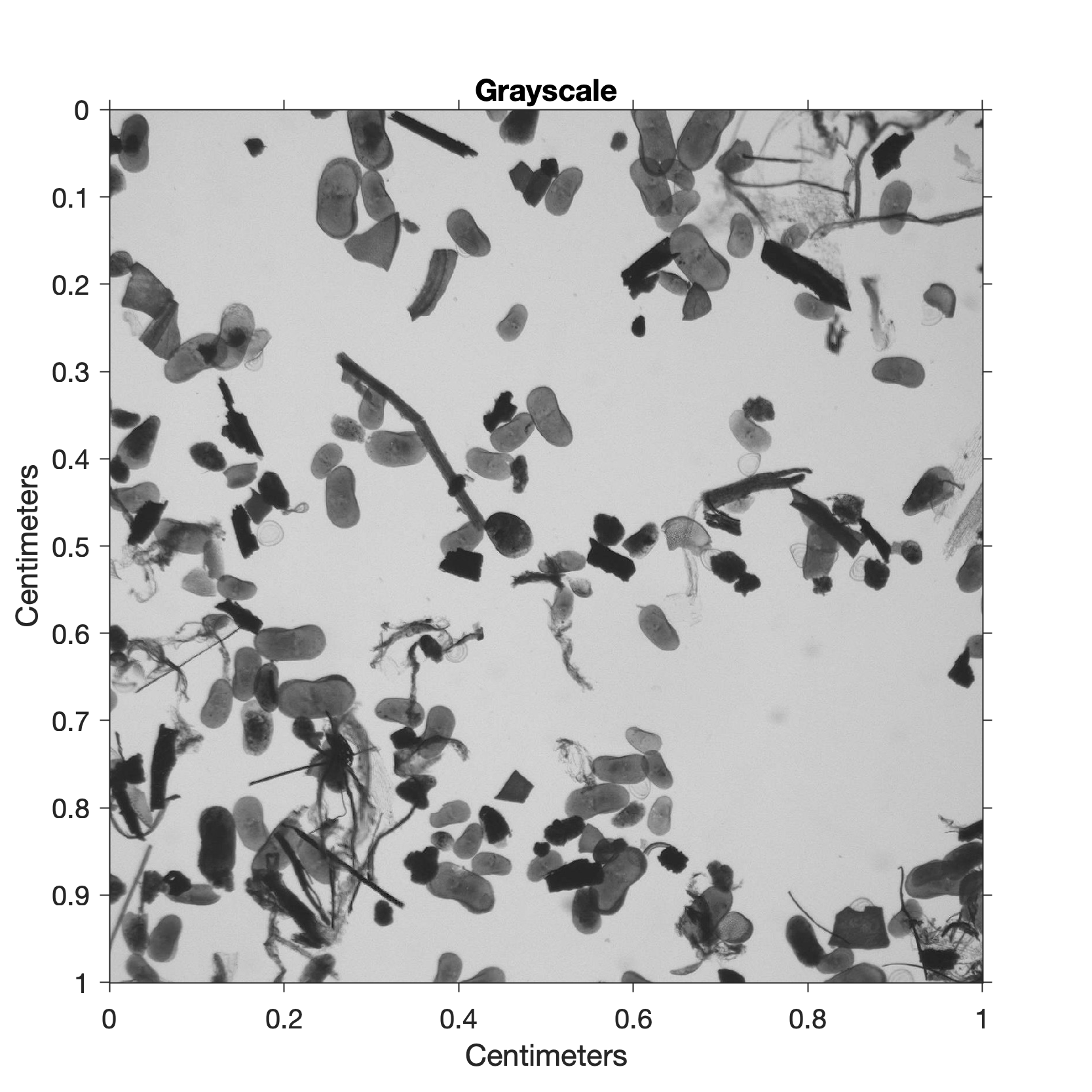
The RGB color image is then converted to a grayscale image using the function rgb2gray:
I2 = rgb2gray(I1);

imshow(I2,...
   'XData',[0 ix],...
   'YData',[0 iy]), axis on
xlabel('Centimeters')
ylabel('Centimeters')
title('Grayscale')
Since the image contrast is relatively low, we use the function imadjust to adjust the image intensity values. The function imadjust maps the values in the intensity image I1 to new values in I2, such that 1% of the data is saturated at low and high intensities of I2. This increases the contrast in the new image I3:
I3 = imadjust(I2);

imshow(I3,...
   'XData',[0 ix],...
   'YData',[0 iy]), axis on
xlabel('Centimeters')
ylabel('Centimeters')
title('Better Contrast')

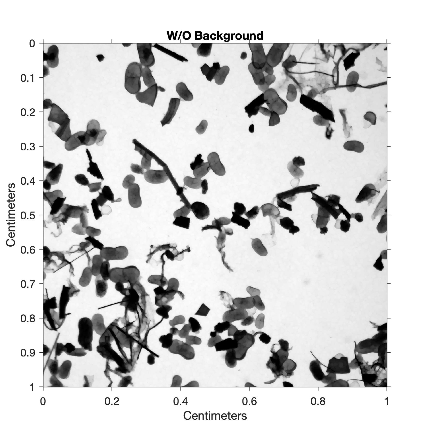
We next determine the background of the image. The function imopen(im,se) determines objects in an image im below a certain pixel size and a flat structuring element se, such as a disk with a radius of 5 pixels generated by the function strel. The variable I4 is the background-free image resulting from this operation.
I4 = imopen(I3,strel('disk',5));

imshow(I4,...
   'XData',[0 ix],...
   'YData',[0 iy]), axis on
xlabel('Centimeters')
ylabel('Centimeters')
title('W/O Background')
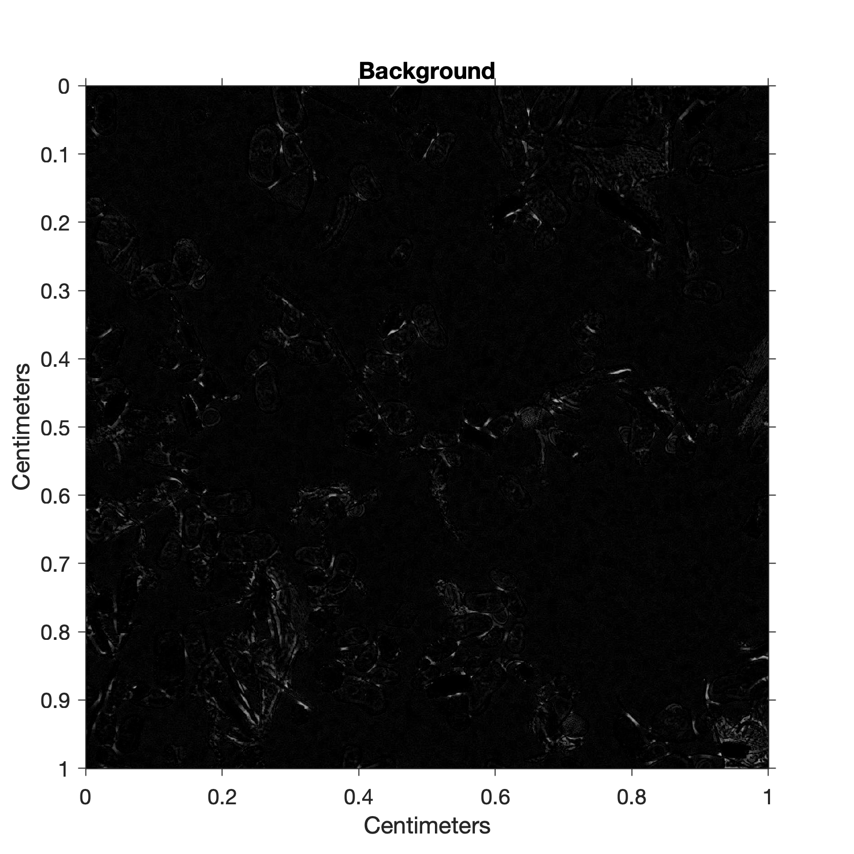
We subtract the background-free image I4 from the original grayscale image I3 to observe the background I5 that has been eliminated.
I5 = imsubtract(I3,I4);

imshow(I5,...
   'XData',[0 ix],...
   'YData',[0 iy]), axis on
xlabel('Centimeters')
ylabel('Centimeters')
title('Background')
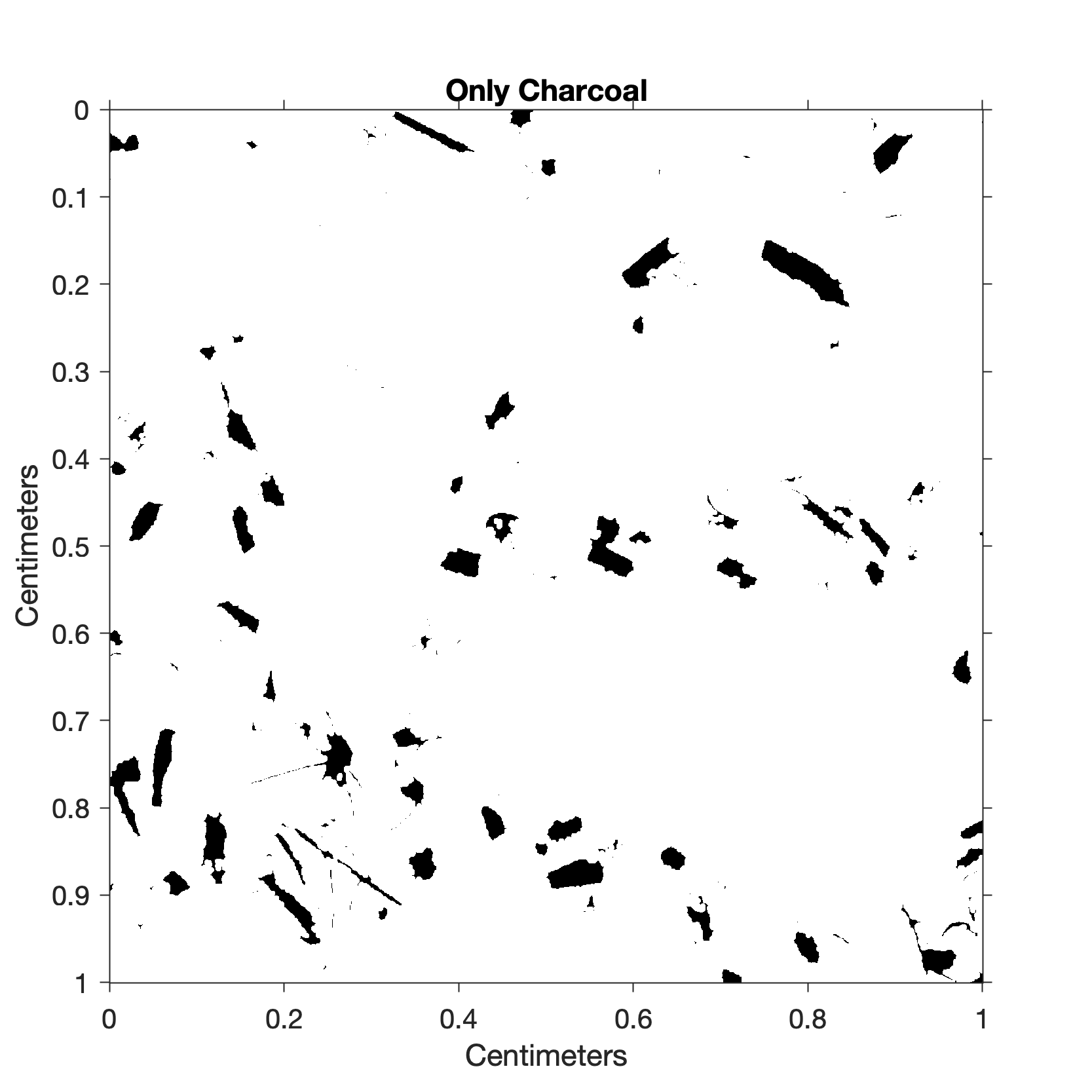
The function im2bw converts the image I4 to a binary image I6 via thresholding. If the threshold is 1.0, the image is all black, corresponding to a pixel value of 0, whereas if the threshold is 0.0, the image is all white, corresponding to a pixel value of 1. We manually change the threshold value until we get a reasonable result. In our example, a threshold of 0.03 produces good results for identifying charcoal fragments:
I6 = im2bw(I4,0.03);

imshow(I6,...
   'XData',[0 ix],...
   'YData',[0 iy]), axis on
xlabel('Centimeters')
ylabel('Centimeters')
title('Only Charcoal')
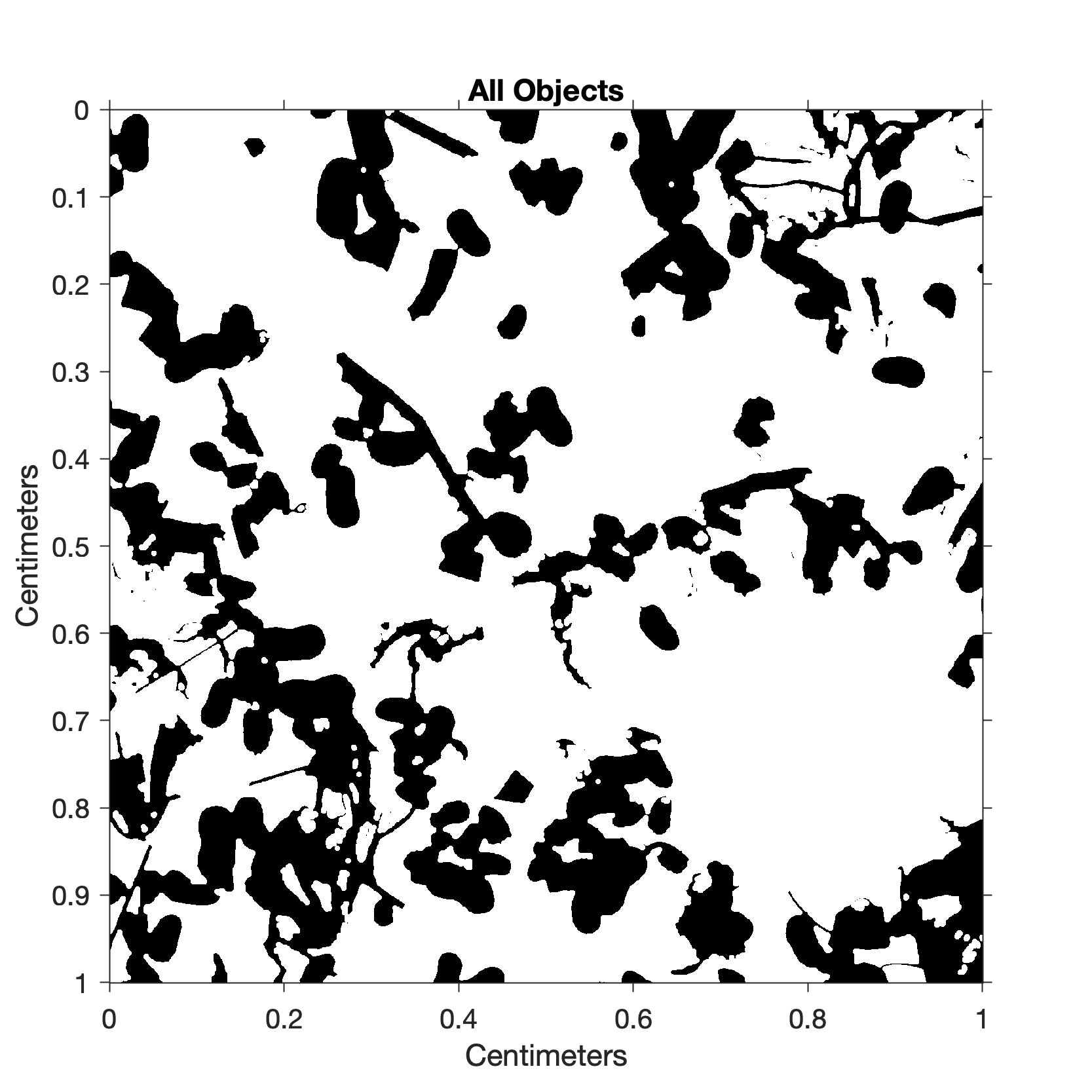
I7 = im2bw(I4,0.6);

figure('Position',[50 300 400 400],...
   'Color',[1 1 1])
axes('Position',[0.1 0.1 0.8 0.8])
imshow(I7,...
   'XData',[0 ix],...
   'YData',[0 iy]), axis on
xlabel('Centimeters')
ylabel('Centimeters')
title('All Objects')
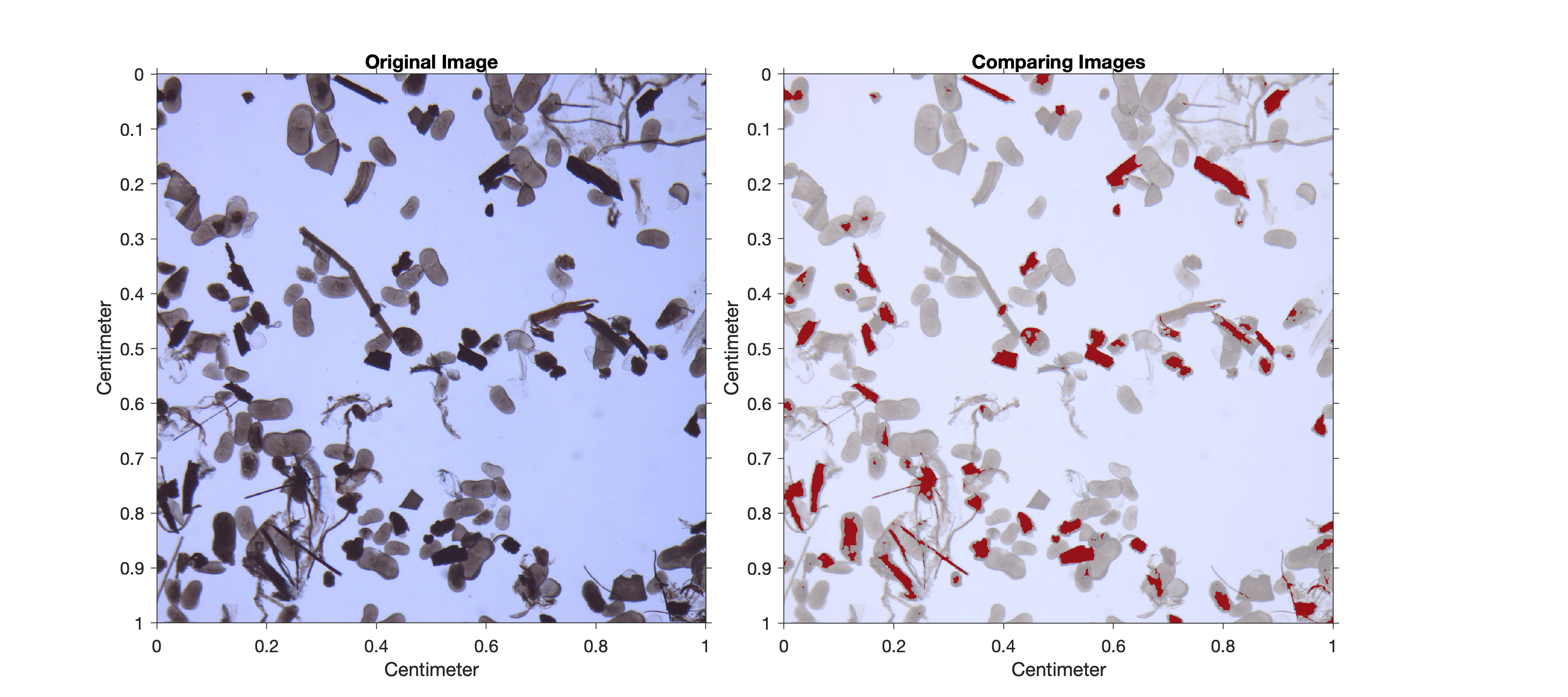
imshow(I1,...
   'XData',[0 ix],...
   'YData',[0 iy]), axis on
xlabel('Centimeters')
ylabel('Centimeters')
title('Original Image')
axes('Units','Normalized',...
   'Position',[0.5 0.1 0.35 0.8])
RA = imref2d(size(I1),[0 ix],[0 iy]);
imshowpair(I6,RA,I7,RA,'blend')
xlabel('Centimeters')
ylabel('Centimeters')
title('Comparing Images')
I8 = 255 * repmat(uint8(I6),1,1,3);
I8(1,:,:) = 255;
I8(:,:,1) = 255;

imshow(I1,...
   'XData',[0 ix],...
   'YData',[0 iy]), axis on
xlabel('Centimeters')
ylabel('Centimeters')
title('Original Image')
axes('Units','Normalized',...
   'Position',[0.5 0.1 0.35 0.8])
RA = imref2d(size(I1),[0 ix],[0 iy]);
imshowpair(I1,RA,I8,RA,'blend')
xlabel('Centimeters')
ylabel('Centimeters')
title('Comparing Images')
We are not interested in the absolute area of charcoal in the image, but rather in the percentage of charcoal in the sample. Typing
100*sum(sum(I6==0))/sum(sum(I7==0))
therefore yields
ans =

   13.4063
This result suggests that approximately 13% of the sieved sample is charcoal. As a next step, we could quantify the other components in the sample (e.g., ostracods or mineral grains) by choosing different threshold values.
References
Trauth, M.H. (2021) MATLAB Recipes for Earth Sciences – Fifth Edition. Springer International Publishing, 517 p., ISBN 978-3-030-38440-1. (MRES)