
A while back I wrote a post about John Aitchison’s Log-Ratio Transformation, Part 1, in the time domain and today Part 2 in the frequency domain. Here’s Part 3 with a MATLAB demonstration of a nice Aitchison example presented in an extended abstract by Pawlowsky-Glahn and Egozcue (2013).
In their article (in German) the authors show spurious correlations and countermeasures in the sense of J. Aitchison in a three-component system Sand, Lehm, Ton (engl. sand, loam, clay), with a dilution effect by Wasser (engl. water). To reproduce the example in MATLAB, we first clear the workspace and create colors for plotting.
clear, clc, close all

colors = [
   0 114 189
   217 83 25
   237 177 32
   126 47 142
]./255;
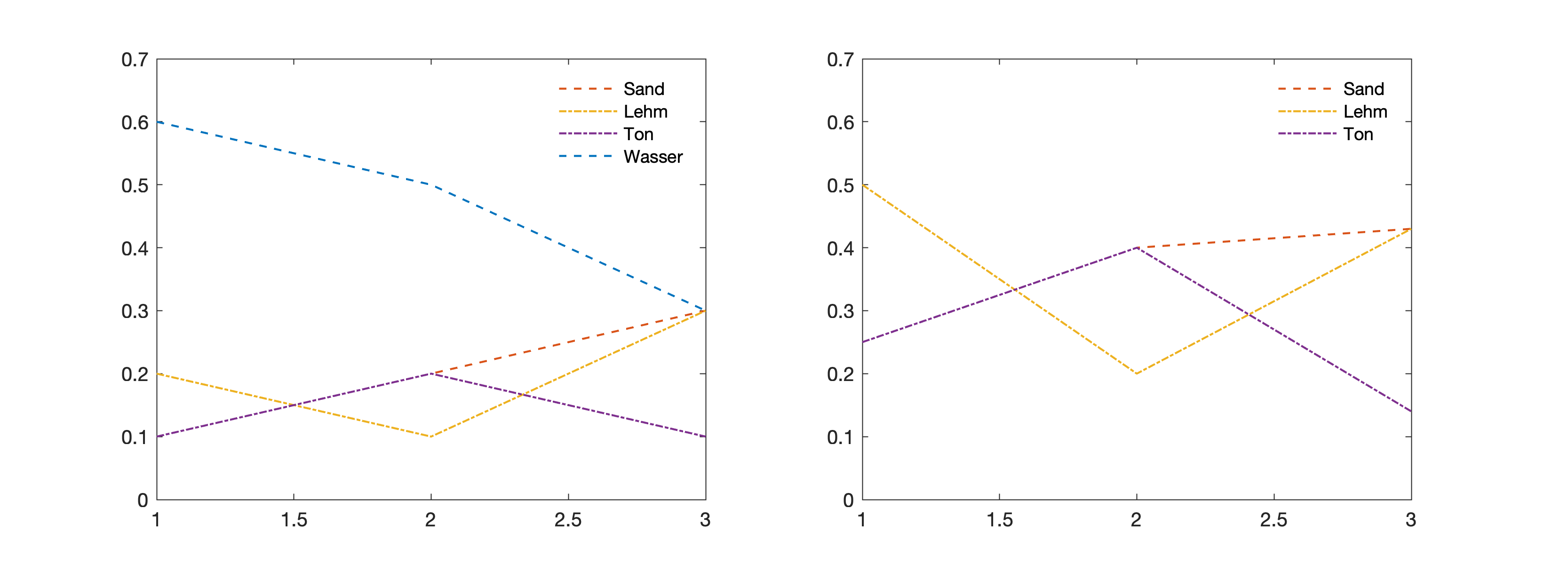
According to the authors, we have the samples in the rows of the arrays, the columns are Sand, Lehm, Ton, Wasser in the data set of Scientist A, but only Sand, Lehm, Ton in the data set of Scientist B. Both A and B get the same values for Sand, Lehm and Ton, but after normalizing it to one Sand and Lehm are positively correlated in A and negatively correlated in B.
According to my interpretation, however, due to the dilution effect of decreasing amount of Wasser in samples 1 to 3 in the analysis of Scientist A, Sand and Lehm together have a positive trend, that is slightly rotated towards a negative trend in the analysis of Scientist B after removing the Wasser content, i.e., normalizing to 1 including and excluding Wasser after drying has a different effect.
A = [
   0.1 0.2 0.1 0.6
   0.2 0.1 0.2 0.5
   0.3 0.3 0.1 0.3
];

B = [
   0.25 0.50 0.25
   0.40 0.20 0.40
   0.43 0.43 0.14
];
We can calculate the correlation coefficients by typing
corr(A(:,1),A(:,2))
corr(B(:,1),B(:,2))
which shows the different signs of the correlation coefficients in the data set of Scientist A and Scientist B.
ans =

   0.5000

ans =

   -0.5583
We can display the data by typing
figure('Position',[100 1000 800 300])
axes('Position',[0.1 0.15 0.35 0.75],...
   'Box','On',...
   'YLim',[0 0.7])
line(1:3,A(:,1),...
   'Color',colors(2,:),...
   'LineWidth',1,...
   'LineStyle','--')
line(1:3,A(:,2),...
   'Color',colors(3,:),'LineWidth',1,...
   'LineStyle','-.')
line(1:3,A(:,3),...
   'Color',colors(4,:),'LineWidth',1,...
   'LineStyle','-.')
line(1:3,A(:,4),...
   'Color',colors(1,:),...
   'LineWidth',1,...
   'LineStyle','--')
legend('Sand','Lehm','Ton','Wasser',...
   'Location','NorthWest',...
   'Box','Off')
axes('Position',[0.55 0.15 0.35 0.75],...
   'Box','On',...
   'YLim',[0 0.7])
line(1:3,B(:,1),...
   'Color',colors(2,:),...
   'LineWidth',1,...
   'LineStyle','--')
line(1:3,B(:,2),...
   'Color',colors(3,:),...
   'LineWidth',1,...
   'LineStyle','-.')
line(1:3,B(:,3),...
   'Color',colors(4,:),...
   'LineWidth',1,...
   'LineStyle','-.')
legend('Sand','Lehm','Ton',...
   'Location','SouthWest',...
   'Box','Off')
We can see this effect by calculating the correlation matrix (the values in Tab 2, B are slightly different in the paper).
corr_A = corrcoef(A)
corr_B = corrcoef(B)
which yields
corr_A =

   1.0000   0.5000   0.0000   -0.9820
   0.5000   1.0000  -0.8660   -0.6547
   0.0000  -0.8660   1.0000    0.1890
  -0.9820  -0.6547   0.1890    1.0000


corr_B =

   1.0000   -0.5583   -0.0675
  -0.5583    1.0000   -0.7901
  -0.0675   -0.7901    1.0000
As said above the joint positive trend of Sand and Lehm in the analysis of Scientist A is removed after removing the negative trend in Wasser content through drying the samples by Scientist B. We correct the dilution effect by calculating the log-ratios according to the principles of John Aitchison
lrA(:,1) = log(A(:,1)./A(:,2));
lrA(:,2) = log(A(:,1)./A(:,3));
lrA(:,3) = log(A(:,2)./A(:,3));

lrB(:,1) = log(B(:,1)./B(:,2));
lrB(:,2) = log(B(:,1)./B(:,3));
lrB(:,3) = log(B(:,2)./B(:,3));
and display the data by typing
figure('Position',[100 600 800 300])
axes('Position',[0.1 0.15 0.35 0.75],...
   'Box','On',...
   'YLim',[0 3])
line(1:3,lrA(:,1),...
   'Color',colors(2,:),...
   'LineWidth',1,...
   'LineStyle','--')
line(1:3,lrA(:,2),...
   'Color',colors(3,:),...
   'LineWidth',1,...
   'LineStyle','-.')
line(1:3,lrA(:,3),...
   'Color',colors(4,:),...
   'LineWidth',1,...
   'LineStyle','-.')
legend('Sand','Lehm','Ton',...
   'Location','NorthWest',...
   'Box','Off')
axes('Position',[0.55 0.15 0.35 0.75],...
   'Box','On',...
   'YLim',[0 3])
line(1:3,lrB(:,1),...
   'Color',colors(2,:),...
   'LineWidth',1,...
   'LineStyle','--')
line(1:3,lrB(:,2),...
   'Color',colors(3,:),...
   'LineWidth',1,...
   'LineStyle','-.')
line(1:3,lrB(:,3),...
   'Color',colors(4,:),...
   'LineWidth',1,...
   'LineStyle','-.')
legend('Sand','Lehm','Ton',...
   'Location','SouthWest',...
   'Box','Off')
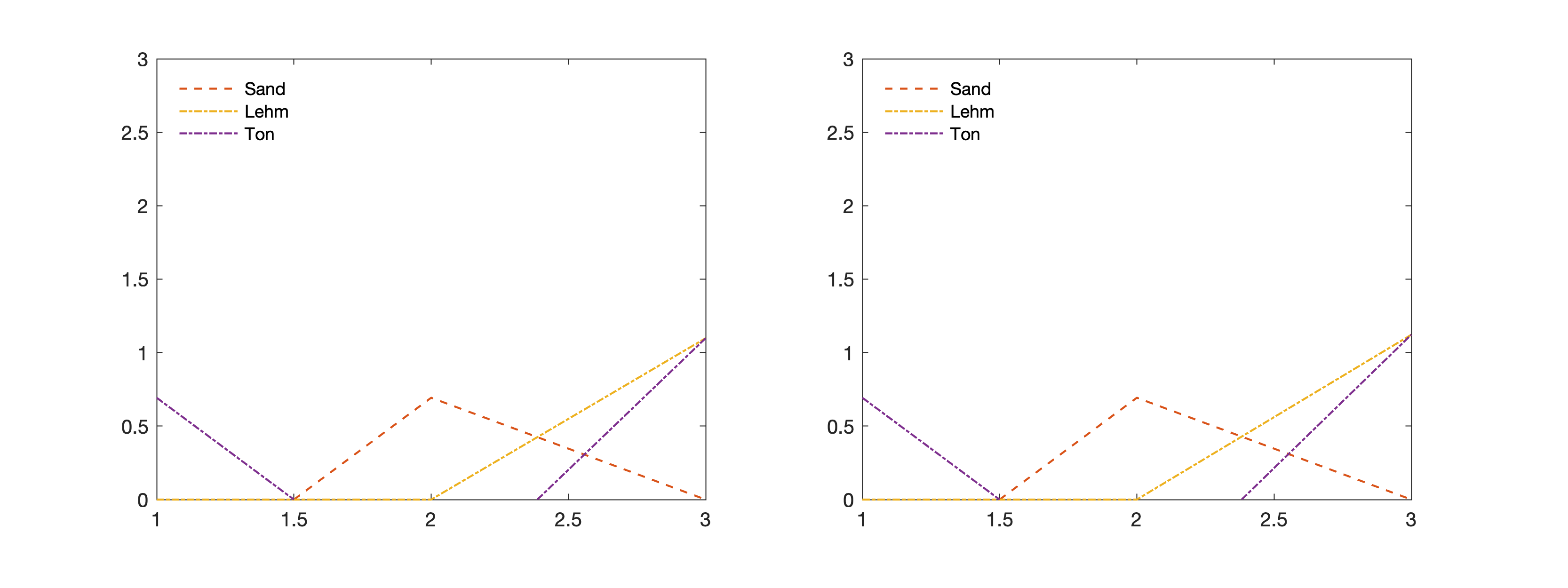
As we see the data sets are now identical with no differences in the correlations. We can also test this by calculating the correlation matrices of log-ratios that almost identical: we get the same (true) correlations.
corr_lrA = corrcoef(lrA)
corr_lrB = corrcoef(lrB)
which yields
corr_lrA =

   1.0000         0   -0.7377
   0         1.0000    0.6751
  -0.7377    0.6751    1.0000


corr_lrB =

   1.0000         0   -0.7306
   0         1.0000    0.6828
  -0.7306    0.6828    1.0000
References:
Aitchison, J., 1986, 2003, The Statistical Analysis of Compositional Data. Blackburn PR, 460 pages.
Aitchison, J., 1999, Logratios and natural laws in compositional data analysis, Mathematical Geology, 31, 563-580.
Pawlowsky-Glahn, V., Egozcue, J.J., Tolosana-Delgado, R., 2007, Lecture Notes on Compositional Data Analysis. (Link)
Pawlowsky-Glahn, V., Egozcue, J.J., 2013, Statistische Analyse von Kompositionsdaten. 58. Berg- und Hüttenmännischer Tag: GIS – Geowissenschaftliche Anwendungen und Entwicklungen. Abstract Volume, 253–360. (Link)