
The Global 30 Arc-Second Elevation Data (GTOPO30) is a 30 arc second (approximately 1 km) global digital elevation data set that contains only elevation data and no bathymetry. MathWorks announced that the gtopo30 function to read the data would be discontinued and that one should use the readgeoraster function instead. Here’s the updated recipe from Chapter 7 of the MRES book (Trauth, 2021).
The Global 30 Arc-Second Elevation Data (GTOPO30) has been developed by the Earth Resources Observation System Data Center and is available from the USGS EarthExplorer website
https://earthexplorer.usgs.gov
As an example we enter the coordinates of the Suguta Valley in the Northern Kenya Rift: 2°8’37.58″N 36°33’47.06″E that can be downloaded using this link. We can use the MATLAB unzip function to decompress the file gt30e020n40_dem.zip, as follows
clear, clc, close all
unzip('gt30e020n40_dem.zip')
After decompressing the zip file we obtain eight files containing the raw data and header files in various formats. The file also provides a GIF image of a shaded relief display of the data. The binary file containing the digital elevation model extracted from gt30e020n40_dem.zip is named gt30e020n40.dem but the old function gtopo30 expects the file to be named E020N40.dem. After rename the files by removing gt30 from the file name in the unzipped collection and use
latlim = [-5 5]; lonlim = [30 40];
GTOPO30 = gtopo30('E020N40',1,latlim,lonlim);
to import the data. The coordinate system is defined using the lon/lat limits listed above. The resolution is 30 arc seconds, corresponding to 1/120 of a degree.
[LON,LAT] = meshgrid(30:1/120:40-1/120,-5:1/120:5-1/120);
We need to reduce the upper limits by 1/120 in order to obtain a matrix of similar dimensions to the GTOPO30 matrix. A grayscale image can be generated from the elevation data using the function surf. The fourth power of the colormap gray is used to darken the map and the colormap is then flipped vertically in order to obtain dark colors for high elevations and light colors for low elevations, instead of the other way around.
surf(LON,LAT,GTOPO30)
shading interp
colormap(flipud(gray.^4))
axis equal, view(0,90)
colorbar
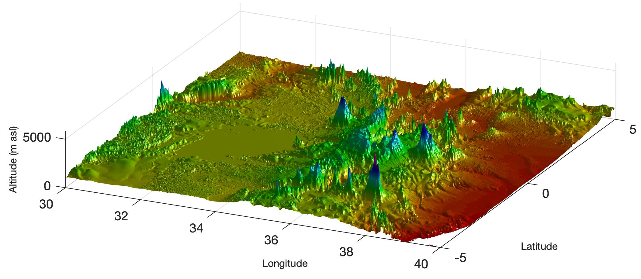
This script opens a new Figure Window and generates the gray surface using interpolated shading, displayed in an overhead view. We also can plot the digital topography as a surface plot with angled lighting.
clf
axes('Visible','off')
surf(LON,LAT,GTOPO30,...
    'SpecularExponent',20,...
    'FaceLighting','phong',...
    'FaceColor','interp',...
    'EdgeColor','none');
light('Style','local',...
    'Position',[145 70 155801])
set(gca,'View',[25 20])
colormap hsv
daspect([1 1 4000])
title('GTOPO30 Data Set',...
    'FontSize',10)
xlabel('Longitude',...
    'FontSize',8)
ylabel('Latitude',...
    'FontSize',8)
zlabel('Altitude (m asl)',...
    'FontSize',8)
We again export the graph as a PNG file
print -dpng -r300 gtopo30.png
with a resolution of 300 dpi. During the writing of the book, it was announced that the gtopo30 function would be discontinued and that one should use the readgeoraster function instead. The MATLAB script to load the data set using the new function is
clear, close all, clc
[A,R] = readgeoraster('e020n40.dem',...
    'OutputType','uint16');
The following series of commands
geoshow(A,R,...
    'DisplayType','texturemap')
colormap(flipud(gray.^4))
set(gca,'XLim',[30 40],...
    'YLim',[-5 5])
helps to create a graph that corresponds to the first of the two graphs above. The function geoshow provides many options to be used to change the appearance of the graphic.
References
Trauth, M.H. (2021) MATLAB Recipes for Earth Sciences – Fifth Edition. Springer International Publishing, ~500 p., Supplementary Electronic Material, Hardcover, ISBN: 978-3-030-38440-1.