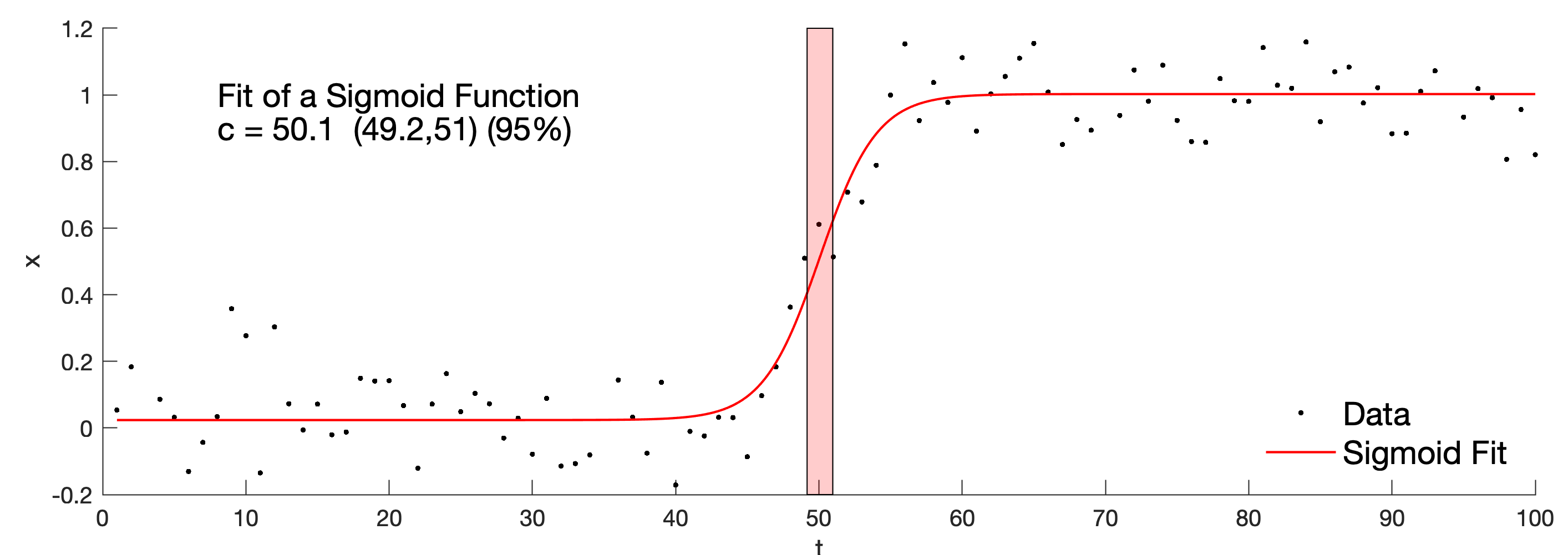
Detecting climate transitions, their relative duration and midpoint, together with confidence bounds, is an important application of time series analysis methods. Here is a MATLAB example of a nonlinear fit of a sigmoid function to noisy data with a transition.
A number of methods are available to detect transitions in climate time series. An example of such methods suitable for use in climate time series is the rampfit method (Mudelsee and Stattegger 1997, Mudelsee 2000), and examples suitable for use in the frequency domain are the evolutionary power spectrum and the wavelet power spectrum (e.g. Lau and Weng 1995, Mackenzie et al. 2001, Trauth, 2020). Here is another way to describe a transition with a sigmoid function, performed with the function fit in MATLAB.
We can analyze time series for the amplitude, duration and midpoint of a climate transition using a fit of a sigmoid function with m = 4 parameters a, b, c, and d
to the records x(t) with n data points using nonlinear least squares fitting. The sigmoid function is a monotonic s-shaped curve, often referred to as a smooth version of a step function. The sigmoid function is bounded by two horizontal asymptotes. It has a bell-shaped first derivative and exactly one inflection point (parameter c), which can be interpreted as the midpoint of the transition. To examine the goodness-of-fit statistics we can use the root mean squared error
computed from the residual MSE, which is in turn calculated by dividing the summed square of residuals SSE
by the degrees of freedom v = n – m. The following MATLAB example demonstrates the method on a synthetic dataset. This data sets comprises 100 data points y for the period from t = 0 to t = 100, with a linear transition from y = 0 to y = 1 with a midpoint at t = 50. We use fit together with fitoptions and fittype from the Curve Fitting Toolbox (MathWorks, 2020) of MATLAB to conduct a nonlinear least squares fit of a sigmoid to the data. As the result we get the coefficients a,b, c,d of our model f(x) = a+b*(1./(1+exp(-d*(x-c)))) together with the individual 95% confidence levels.
We first clear the workspace and the Command Window, and close all Figure Windows.
clear, close all, clc
The linear transition within the synthetic time series starts at t = 46 and ends at t = 55, and has a slope of 1/10 and a y-intercept of –4.5. The Gaussian noise has a mean of 0 and a standard deviation of 0.1. Such a data set can be generated with the following MATLAB script:
rng(0)
data(1:100,1) = 1 : 1 : 100;
data(1:45,2) = 0;
data(46:55,2) = 1/10 * data(46:55,1) - 4.5;
data(56:100,2) = 1;
data(:,2) = data(:,2) + 0.1*randn(size(data(:,2)));
These synthetic data sets were then analyzed using the function fit together with fitoptions and fittype to perform the nonlinear least square fitting. We fit a sigmoid function with four parameters a, b, c, and d, whose starting values we first define together with NonlinearLeastSquares using fitoptions:
fo = fitoptions('Method','NonlinearLeastSquares',...
    'StartPoint',[0 1 50 1]);
Next we define the model a+b*(1./(1+exp(-d*(x-c)))) in fittype using
ft = fittype(@(a,b,c,d,x) a+ ...
    b*(1./(1+exp(-d*(x-c)))),...
    'Coeff',{'a','b','c','d'},...
    'Options',fo);
We then use fit to find the best values for a, b, c, and d in a least-squares sense.
f = fit(data(:,1),data(:,2),ft)
which yields estimates of the four parameters including their 95% confidence bounds:
f =

General model:
ft(a,b,c,d,x) = a+b*(1./(1+exp(-d*(x-c))))
Coefficients (with 95% confidence bounds):
     a = 0.02369 (-0.01299, 0.06038)
     b = 0.9788 (0.9264, 1.031)
     c = 50.07 (49.17, 50.97)
     d = 0.5025 (0.3052, 0.6998)

gof =

  struct with fields:

     sse: 1.3848
     rsquare: 0.9409
     dfe: 96
     adjrsquare: 0.9390
     rmse: 0.1201

output =

  struct with fields:

     numobs: 100
     numparam: 4
     residuals: [100×1 double]
     Jacobian: [100×4 double]
     exitflag: 3
     firstorderopt: 0.0010
     iterations: 14
     funcCount: 75
     cgiterations: 0
     algorithm: 'trust-region-reflective'
     stepsize: 0.0017
     message: 'Success, but fitting stopped
     because change in residuals less than
     tolerance (TolFun).'
which includes the root mean squared error rmse. We then extract the regression coefficients and confidence bounds ci using
cv = coeffvalues(f);
ci = confint(f,0.95);
cs = ['c = ',num2str(cv(1,3),3),' (', ...
num2str(ci(1,3),3),',', ...
num2str(ci(2,3),3),') (95%)'];
and display the result by typing
figure('Position',[50 1100 800 250])
axes('XLim',xl,'YLim',yl), hold on
p = plot(f,data(:,1),data(:,2));
p(2).LineWidth = 1;
p(1).Color = [0 0 0];
patch('Faces',[1 2 3 4],...
   'Vertices',[ci(1,3) -.2; ci(2,3) -.2; ...
    ci(2,3) 1.2; ci(1,3) 1.2],...
   'FaceColor',[1 0 0],...
   'FaceAlpha',.2)
text(8,1,'Fit of a Sigmoid Function',...
   'FontSize',14)
text(8,0.9,cs,...
   'FontSize',14)
xlabel('t'), ylabel('x')
lgd = legend('Data','Sigmoid Fit');
lgd.FontSize = 14;
lgd.Location = 'southeast';
lgd.Box = 'Off';
The fitted sigmoid function can now be used to determine the duration of the climate transition. It can also be used to determine the mid point of the transition, along with the 95% confidence interval marked by a red bar.
References
Lau KM, Weng H (1995) Climate Signal Detection Using Wavelet Transform: How to Make a Time Series Sing. Bulletin of the American Meteorological Society 76:2391–2402
Mackenzie D, Daubechies I, Kleppner D, Mallat S, Meyer Y, Ruskai MB, Weiss G (2001) Wavelets: Seeing the Forest and the Trees. Beyond Discovery, National Academy of Sciences, December 2001, available online at http://www.beyonddiscovery.org
MathWorks, 2020. Curve Fitting ToolboxTM User’s Guide. The MathWorks, Inc., Natick, MA.
Mudelsee M, Stattegger M (1997) Exploring the structure of the mid-Pleistocene revolution with advanced methods of time-series analysis. International Journal of Earth Sciences 86:499–511
Mudelsee M (2000) Ramp function regression: A tool for quantifying climate transitions. Computers and Geosciences 26:293–307
Trauth, M.H. (2020) MATLAB Recipes for Earth Sciences – Fifth Edition. Springer International Publishing, 517 p., Supplementary Electronic Material, Hardcover, ISBN: 978-3-030-38440-1


