
Computing the evolutionary spectrum of a short piano piece helps to recognize that music is the result of a complex interplay of temporal and spectral changes of sound. The MATLAB Audio Toolbox has numerous useful functions for spectrally analyzing music.
In this experiment, we will look at music in both the time and frequency domains. We mainly represent signals in the time domain in order to look at a temporal variation of the amplitude of the signal. The spectral decomposition of the signal into harmonic components, on the other hand, helps to represent the distribution of the information contained in the signal (e.g. the energy, the variance) as a function of periods (or wavelengths) or their reciprocal, the frequencies (or wave numbers). The transition from the time domain to the frequency domain is performed, as examples, by the prism for visible light, the mass spectrometer for atoms and molecules, and the Fourier transform in data analysis.
In this experiment we play a short piece of music on a Yamaha Clavinova CLP-860 (1998) digital piano using the Jazz Piano tone color. The audio signal was recording using the Apple VoiceMemos app on an iPhone 8 and saved in .wav files. We copied the audio files to the computer, moved them to our working folder or any other directory contained in current search path of MATLAB. After clearing the workspace, the command window and close all figures, we read the audio file and play the signal as sound.
clear, close all, clc

x5 = audioread('exercise_7_4_4_data_5.wav');
x5info = audioinfo('exercise_7_4_4_data_5.wav');

sound(x5,48000)
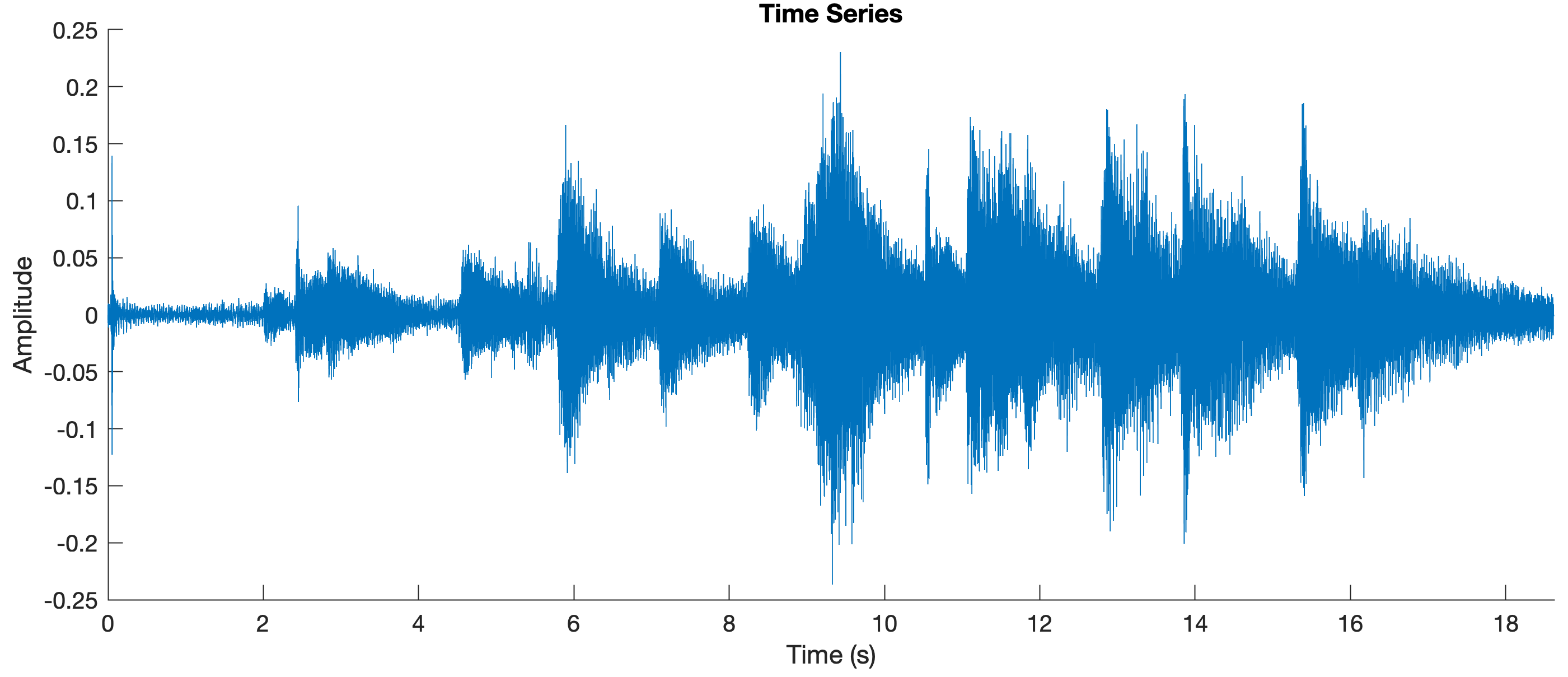
Again we display the signal in the time domain.
figure('Position',[50 1000 800 300],...
   'Color',[1 1 1])
axes('XLim',[0 length(x5)/x5info.SampleRate])
line((1:length(x5))/x5info.SampleRate,x5)
xlabel('Time (s)')
ylabel('Amplitude')
title('Time Series')
where we clearly see the touch of the different keys of the piano.
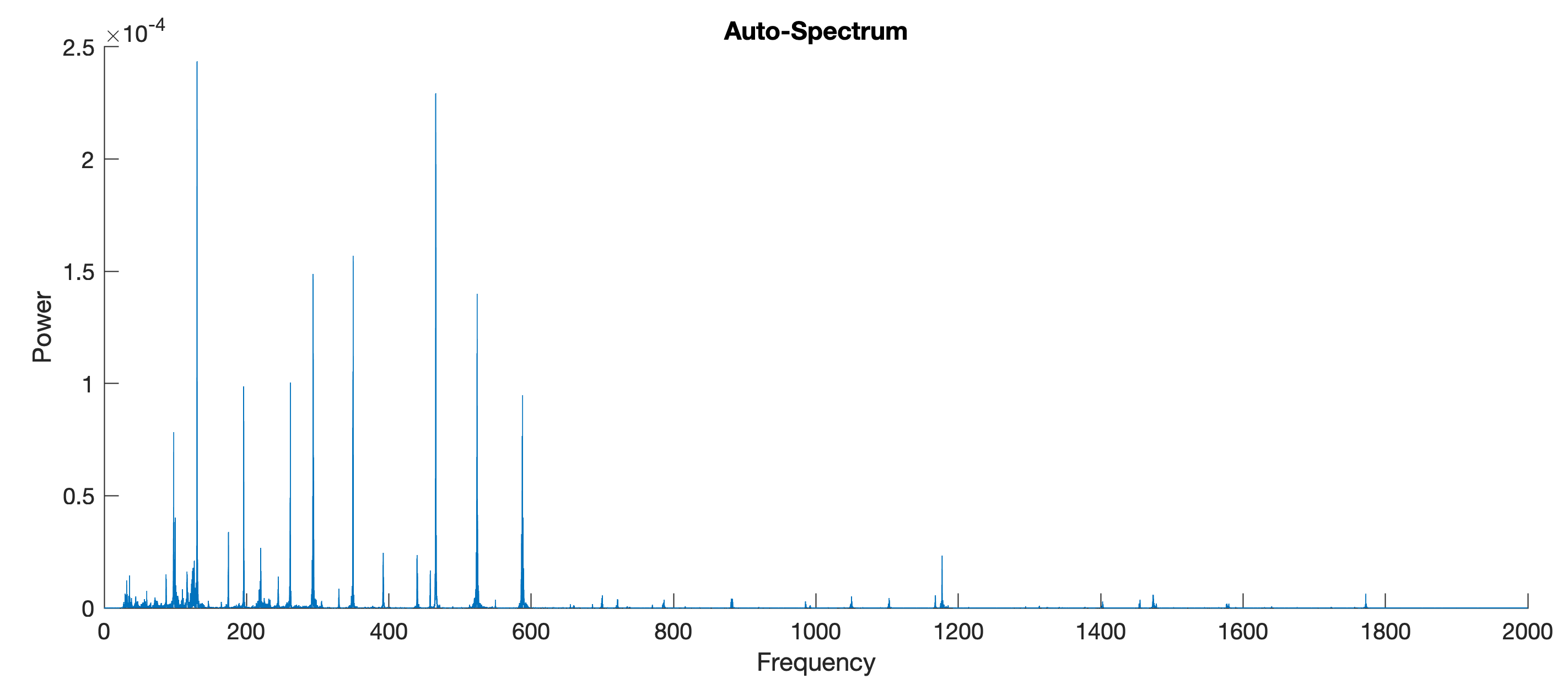
The periodogram again shows the fundamental tone and the overtones
[Pxx5,f5] = ...
   periodogram(x5,[],length(x5),x5info.SampleRate);

figure('Position',[50 600 800 300],...
   'Color',[1 1 1])
axes('XLim',[0 2000])
line(f5,abs(Pxx5))
xlabel('Frequency')
ylabel('Power')
title('Auto-Spectrum')
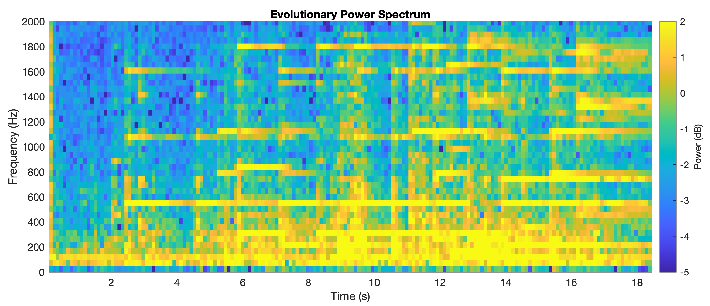
The complexity of the piece of piano music is much better displayed in a spectrogram.
[sn5,fn5,tn5] = ...
   spectrogram(x5,10000,5000,1000,x5info.SampleRate);

figure('Position',[50 200 800 300],...
   'Color',[1 1 1])
pcolor(tn5,fn5,log(abs(sn5))), shading flat
set(gca,'YLim',[0 2000])
title('Evolutionary Power Spectrum')
ylabel('Frequency (Hz)')
xlabel('Time (s)')
caxis([-5 2])
c = colorbar;
c.Label.String = 'Power (dB)';
Here we can see the temporal appearance of tones and overtones, displayed as horizontal strings of yellow and orange pixels in the pseudocolor plot.
Download the MATLAB script and example image.