
 In paleoclimate time series amplitude of spectral peaks usually varies with time. Evolutionary power spectral analysis such as the FFT-based spectrogram and wavelet power spectral analysis helps. These methods, however, require interpolation of the time series to a grid of evenly-spaced times. Instead we can use the Lomb-Scargle Method for unevenly-spaced spectral analysis, computed for a sliding window, to map changes of the cyclicities through time.
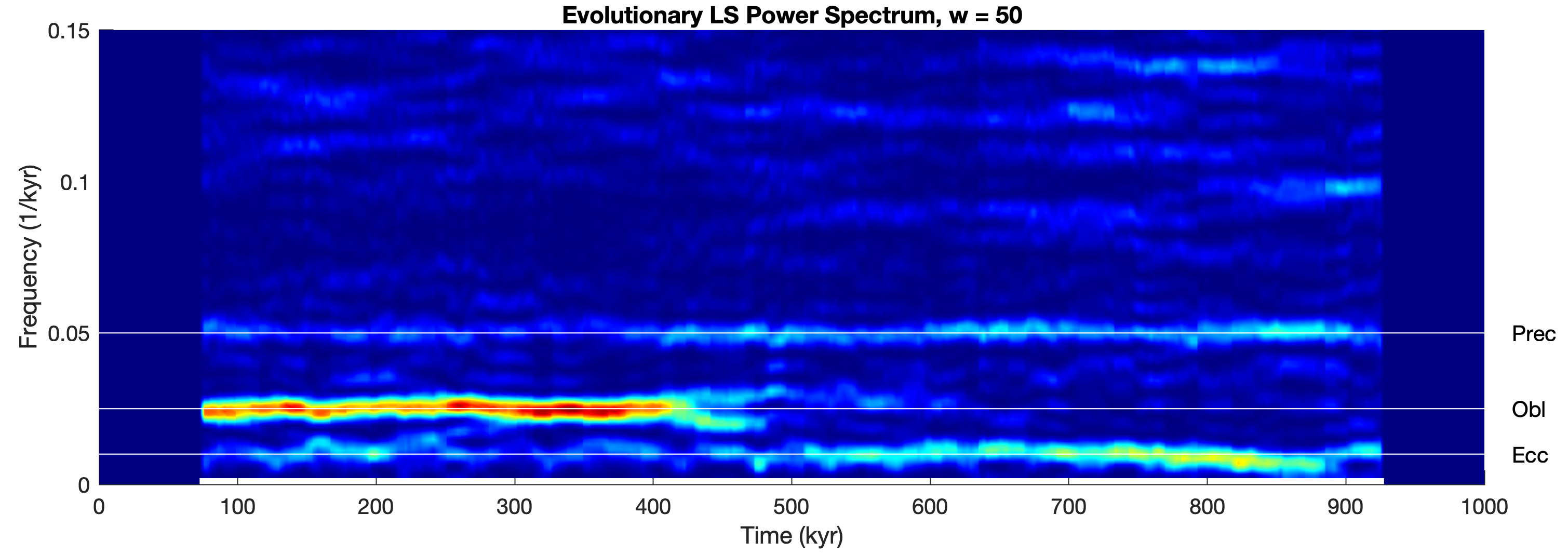
The amplitude of spectral peaks usually varies with time. This is particularly true for paleoclimate time series. Paleoclimate records usually show trends, not only in the mean and variance but also in the relative contributions of rhythmic components such as the Milankovitch cycles in marine oxygen-isotope records. Evolutionary power spectra have the ability to map such changes in the frequency domain.
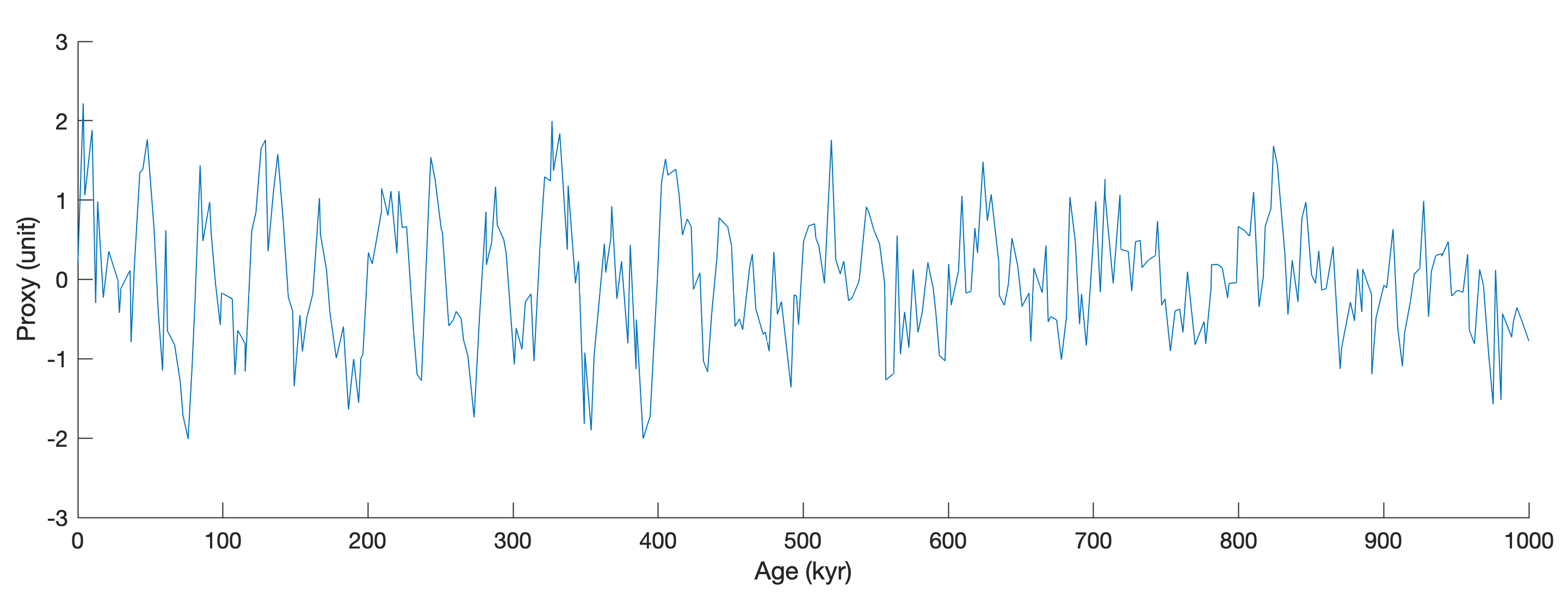
Here is a modification of the code of the Lomb-Scargle method described in Chapter 5 of the MRES book (Trauth 2025) to allow us to compute an evolutionary LS spectrum. We first clear the workspace, determine the display size for scaling the graphics and load the data series3.txt from the MRES book. The data series contains three main periodicities of 100, 40 and 20 kyrs and additive Gaussian noise. The amplitudes, however, change through time and this example can therefore be used to illustrate the advantage of the evolutionary power spectrum method. In our example the 40 kyr cycle appears only after ca. 450 kyrs, whereas the 100 and 20 kyr cycles are present throughout the time series.
clear, clc, close all
ds = get(0,'ScreenSize');
data = load('series3.txt');
We then plot the data.
figure('Position',[50 ds(4)-500 800 300],...
    'Color','w');
axes('Position',[0.1 0.15 0.8 0.7])
line(data(:,1),data(:,2))
xlabel('Age (kyr)')
ylabel('Proxy (unit)')
The data are irregular spaced
figure('Position',[50 ds(4)-600 800 300],...
    'Color','w');
axes('Position',[0.1 0.15 0.8 0.7])
line(data(1:end-1,1),diff(data(:,1)))
xlabel('Age (kyr)')
ylabel('Delta Age (kyr)')
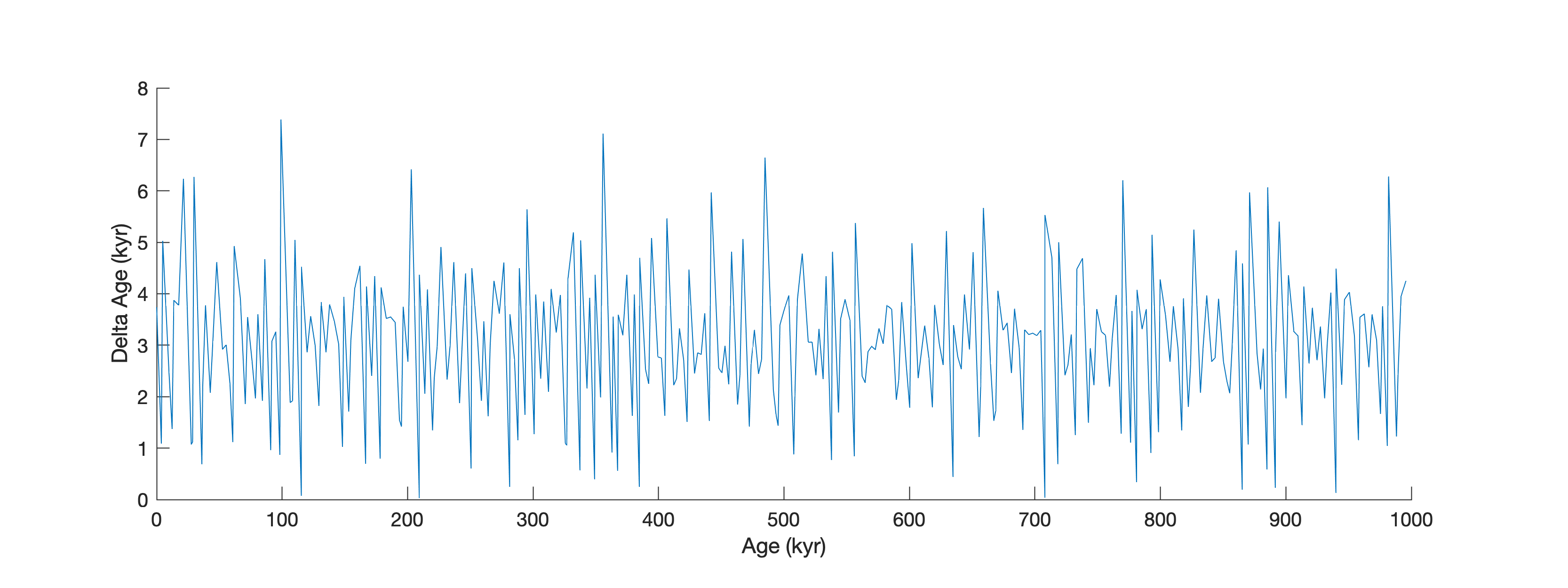
as we can also see when plotting the time differences of subsequent data point in a histogram
figure('Position',[50 ds(4)-700 800 300],...
    'Color','w');
axes('Position',[0.1 0.15 0.8 0.7])
histogram(diff(data(:,1)),20)
xlabel('Age Difference (kyr)')
ylabel('Counts')
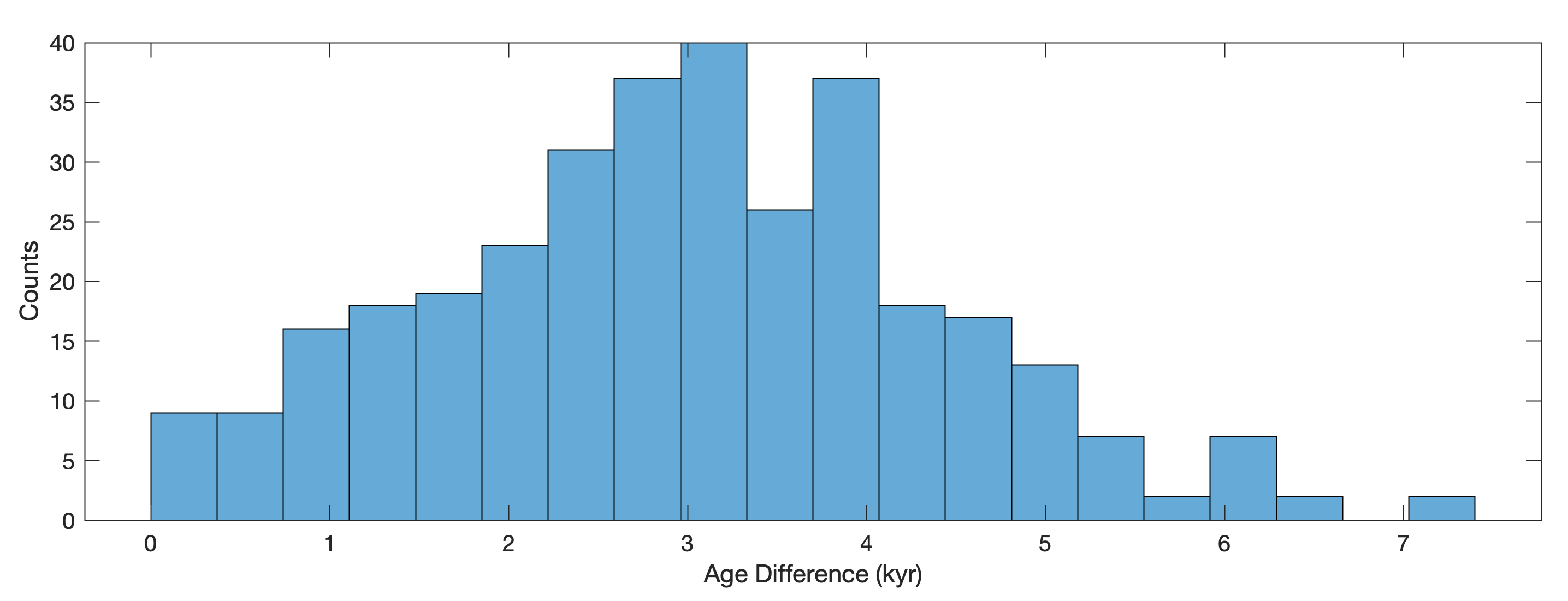
The median of the time differences is
median(diff(data(:,1)))
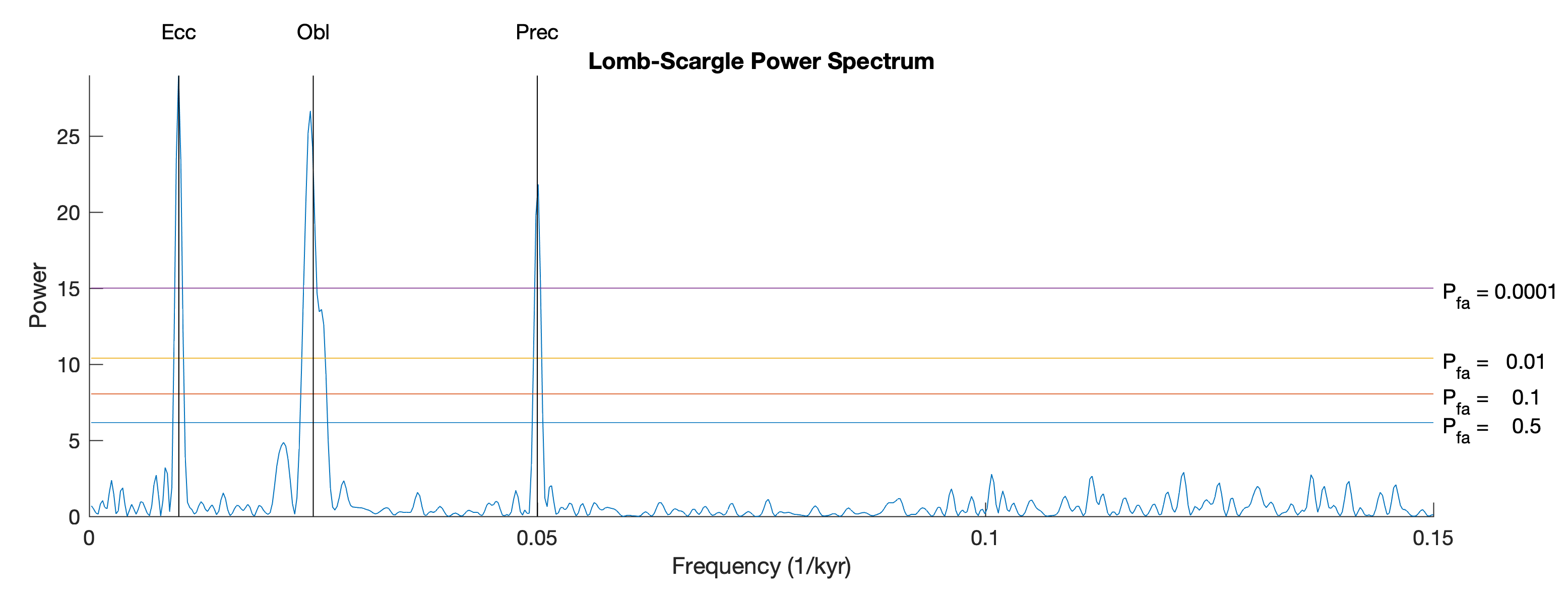
Since the data are unevenly-spaced we use the Lomb-Scargle (LS) Method to compute the power spectrum, described in Chapter 5.7 of the MRES book (Trauth, 2020) but modified to calculate an evoluationary Lomb-Scargle Power Spectrum. We first define the false alarm probability.
Pfa = [50 10 1 0.01]/100;
Pd = 1-Pfa;
The we use the function plomb from the Signal Processing Toolbox (MathWorks, 2025) to calculate the LS power spectrum of the full time series
[pxx,f,pth] = plomb(data(:,2),data(:,1),...
    'normalized','Pd',Pd);
and display the result
figure('Position',[50 ds(4)-800 800 300],...
    'Color','w')
axes('Position',[0.1 0.15 0.8 0.7],...
    'XLim',[0 0.15],...
    'YLim',[0 max(pxx(:))]); hold on
line(f,pxx)
line(f,pth*ones(size(f')))
line([1/20 1/20],...
    [0 max(pxx(:))],...
    'Color','k')
line([1/40 1/40],...
    [0 max(pxx(:))],...
    'Color','k')
line([1/100 1/100],...
    [0 max(pxx(:))],...
    'Color','k')
text(1/20,max(pxx(:))+0.1*max(pxx(:)),...
    'Prec','HorizontalAlignment','center')
text(1/40,max(pxx(:))+0.1*max(pxx(:)),...
    'Obl','HorizontalAlignment','center')
text(1/100,max(pxx(:))+0.1*max(pxx(:)),...
    'Ecc','HorizontalAlignment','center')
text(0.151*[1 1 1 1],pth-.5, ...
    [repmat('P_{fa} = ',[4 1]) num2str(Pfa')])
xlabel('Frequency (1/kyr)')
ylabel('Power')
title('Lomb-Scargle Power Spectrum')
hold off
We then calculate the LS power spectrum of a sliding window of length w. After defining the window size, we pre-allocate memory for the output of plomb and then calculate the LS spectra of the sliding window.
clear pxx f pth
w = 50;

pxxevol = zeros(2*w+2,length(data));
fevol   = zeros(2*w+2,length(data));
pthevol = zeros(4,length(data));

for i = w/2+1 : length(data)-w/2
    clear pxxi fi pthi
    [pxxevol(:,i),fevol(:,i),...
        pthevol(:,i)] = ...
        plomb(data(i-w/2:i+w/2,2),...
        data(i-w/2:i+w/2,1),...
        'normalized','Pd',Pd);
end
We then display the result.
figure('Position',[50 ds(4)-900 800 300],...
    'Color','w')
axes('Position',[0.1 0.15 0.8 0.7],...
    'YLim',[0 0.15],...
    'ZLim',[0 max(pxxevol(:))]), hold on
surf(data(:,1),fevol,pxxevol), shading interp
view(0,90)
plot3([min(data(:,1)) max(data(:,1))],...
    [1/20 1/20],...
    [max(pxxevol(:)) max(pxxevol(:))],'w')
plot3([min(data(:,1)) max(data(:,1))],...
    [1/40 1/40],...
    [max(pxxevol(:)) max(pxxevol(:))],'w')
plot3([min(data(:,1)) max(data(:,1))],...
    [1/100 1/100],...
    [max(pxxevol(:)) max(pxxevol(:))],'w')
text(max(data(:,1))+0.02*max(data(:,1)),...
    1/20,'Prec')
text(max(data(:,1))+0.02*max(data(:,1)),...
    1/40,'Obl')
text(max(data(:,1))+0.02*max(data(:,1)),...
    1/100,'Ecc')
xlabel('Time (kyr)')
ylabel('Frequency (1/kyr)')
titlestr = ...
    ['Evolutionary LS Power Spectrum, w = ',...
    num2str(w)];
title(titlestr)
colormap(jet)
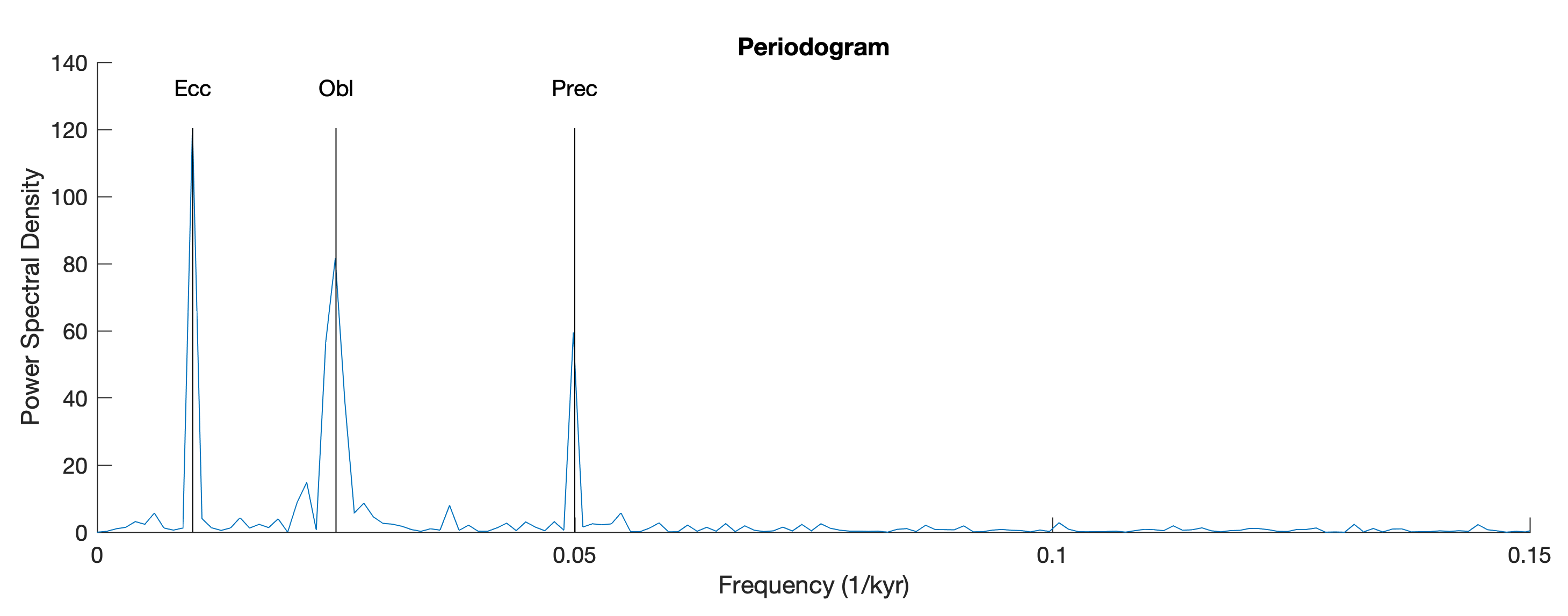
We can then compare the LS power spectrum with an FFT-based periodogram of the full time series which requires interpolation.
tint = min(data(:,1)):...
    (max(data(:,1))-min(data(:,1)))/...
    length(data(:,1)):max(data(:,1));
dataint = interp1(data(:,1),data(:,2),tint,...
    'pchip');

fs = 1/((max(data(:,1))-min(data(:,1)))/...
    length(data(:,1)));

[pfft,ffft] = ...
    periodogram(dataint,[],length(dataint),fs);
We then plot the result.
figure('Position',[50 ds(4)-1000 800 300],...
    'Color','w')
axes('Position',[0.1 0.15 0.8 0.7],...
    'XLim',[0 0.15])
line(ffft,abs(pfft))
line([1/20 1/20],[0 max(pfft(:))],...
    'Color','k')
line([1/40 1/40],[0 max(pfft(:))],...
    'Color','k')
line([1/100 1/100],[0 max(pfft(:))],...
    'Color','k')
text(1/20,max(pfft(:))+0.1*max(pfft(:)),...
    'Prec','HorizontalAlignment','center')
text(1/40,max(pfft(:))+0.1*max(pfft(:)),...
    'Obl','HorizontalAlignment','center')
text(1/100,max(pfft(:))+0.1*max(pfft(:)),...
    'Ecc','HorizontalAlignment','center')
xlabel('Frequency (1/kyr)')
ylabel('Power Spectral Density')
title('Periodogram')
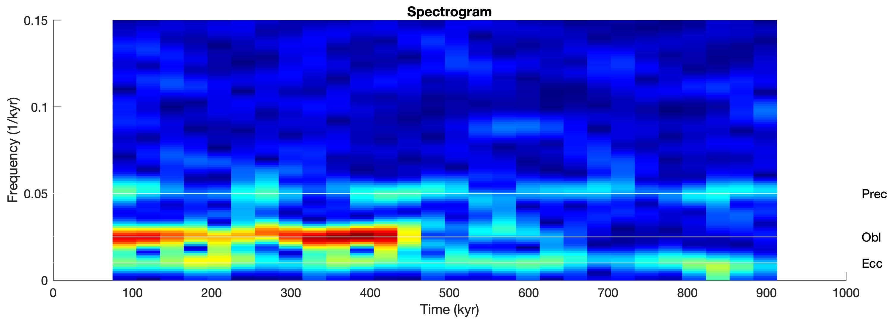
We can compare the result with those of other methods of evolutionary power spectral analysis, such as the FFT-based spectrogram that also requires interpolation. We are using the function spectrogram from the Signal Processing Toolbox (MathWorks, 2025).
[ssp,fsp,tsp] = ...
    spectrogram(dataint,w,w-10,[],fs);

figure('Position',[50 ds(4)-1100 800 300],...
    'Color','w')
axes('Position',[0.1 0.15 0.8 0.7],...
    'XLim',[0 1000],...
    'YLim',[0 0.15]); hold on
pcolor(tsp,fsp,(abs(ssp))), shading flat
line([min(data(:,1)) max(data(:,1))],...
    [1/20 1/20],...
    'Color','w')
line([min(data(:,1)) max(data(:,1))],...
    [1/40 1/40],...
    'Color','w')
line([min(data(:,1)) max(data(:,1))],...
    [1/100 1/100],...
    'Color','w')
text(max(data(:,1))+0.02*max(data(:,1)),...
    1/20,'Prec')
text(max(data(:,1))+0.02*max(data(:,1)),...
    1/40,'Obl')
text(max(data(:,1))+0.02*max(data(:,1)),...
    1/100,'Ecc')
title('Spectrogram')
xlabel('Time (kyr)')
ylabel('Frequency (1/kyr)')
set(gcf,'Colormap',jet)
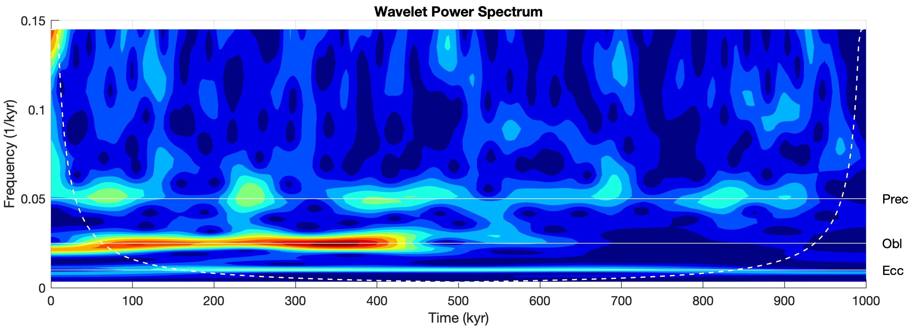
Another method is wavelet power spectral analysis using cwt from the Wavelet Toolbox (MathWorks, 2025) together with the default Morse mother wavelet that also requires interpolation.
[wt,fwt,coi] = cwt(dataint,fs);

figure('Position',[50 ds(4)-1200 800 300],...
'Color','w')
axes('Position',[0.1 0.15 0.8 0.7],...
'YLim',[0 0.15],...
'XGrid','On',...
'YGrid','On'); hold on
contour(tint,fwt,abs(wt),...
'LineStyle','none',...
'LineColor',[0 0 0],...
'Fill','on')
line(tint,coi,'Color','w',...
'LineStyle','--',...
'LineWidth',1)
line([min(data(:,1)) max(data(:,1))],...
[1/20 1/20],...
'Color','w')
line([min(data(:,1)) max(data(:,1))],...
[1/40 1/40],...
'Color','w')
line([min(data(:,1)) max(data(:,1))],...
[1/100 1/100],...
'Color','w')
text(max(data(:,1))+0.02*max(data(:,1)),...
1/20,'Prec')
text(max(data(:,1))+0.02*max(data(:,1)),...
1/40,'Obl')
text(max(data(:,1))+0.02*max(data(:,1)),...
1/100,'Ecc')
xlabel('Time (kyr)')
ylabel('Frequency (1/kyr)')
title('Wavelet Power Spectrum')
set(gcf,'Colormap',jet)
References
Lomb NR (1972) Least-Squared Frequency Analysis of Unequally Spaced Data. Astro-physics and Space Sciences 39:447–462
MathWorks (2025) Signal Processing Toolbox – User’s Guide. The MathWorks, Inc., Natick, MA
Scargle JD (1981) Studies in Astronomical Time Series Analysis. I. Modeling Random Processes in the Time Domain. The Astrophysical Journal Supplement Series 45:1–71
Scargle JD (1982) Studies in Astronomical Time Series Analysis. II. Statistical Aspects of Spectral Analysis of Unevenly Spaced Data. The Astrophysical Journal 263:835–853
Scargle JD (1990) Studies in Astronomical Time Series Analysis. IV. Modeling Chaotic and Random Processes with Linear Filters. The Astrophysical Journal 359:469–482
Scargle JD (1989) Studies in Astronomical Time Series Analysis. III. Fourier Transforms, Autocorrelation Functions, and Cross-Correlation Functions of Unevenly Spaced Data. The Astrophysical Journal 343:874–887
Schulz M, Stattegger K (1998) SPECTRUM: Spectral Analysis of Unevenly Spaced Paleoclimatic Time Series. Computers & Geosciences 23:929–945
Trauth, M.H. (2024) Python Recipes for Earth Sciences – Second Edition. Springer International Publishing, 491 p., https://doi.org/10.1007/978-3-031-56906-7 (PRES)
Trauth, M.H. (2025) MATLAB Recipes for Earth Sciences – Sixth Edition. Springer International Publishing, 567 p, https://doi.org/10.1007/978-3-031-57949-3 (MRES)