
 While updating my book and trying to be as consistent as possible throughout the text and the MATLAB examples I find it quite surprising that the behaviour of graphics function is not consistent in MATLAB.
As an example, according to the docs
data_radians_1 = 4+randn(100,1);
pax = polaraxes('ThetaZeroLocation','top',...
    'ThetaDir','clockwise')
polarhistogram(pax,data_radians_1)
should actually work but we have to add a “hold on” after polaraxes to keep the axes.
data_radians_1 = 4+randn(100,1);
pax = polaraxes('ThetaZeroLocation','top',...
    'ThetaDir','clockwise'), hold on
polarhistogram(pax,data_radians_1)
The reason for that is that polarhistogram creates its own axes, therefore the above series of commands does not work – and the docs do not say that. It’s quite confusing for those getting started with MATLAB I think.
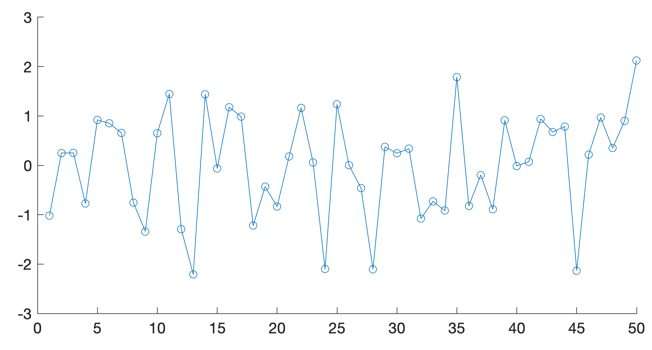
The reason for the inconsistent behaviour is that there are two types of graphics functions in MATLAB: the ones creating their own axes system and others that are actually not graphics functions but they are creating graphics primitives such as lines:
clear
data = randn(100,1);
ax = axes('XLim',[0 50]), hold on
plot(ax,1:length(data),data,...
    'Marker','o')

figure
clear
data = randn(100,1);
ax = axes('XLim',[0 50])
line(ax,1:length(data),data,...
    'Marker','o')
I more and more try to use the root, figure, axis, line system instead of using high level graphics functions. On the other hand, writing the code for a polar histogram is quite time consuming, if you consider that this is only one of many examples in the book and I actually hate polar coordinates!