
Our paleoclimate time series often contain too much detail, i.e. they have a high variance in the high frequency range. Of course, this can be true climate variability, but it usually contains a lot of noise. Therefore we like to plot a filtered variant of the curve together with the original curve and fill the area between the two. Here I show you how it works with MATLAB.
First we create a time series comprising three sinusoidal curves with noise.
t = 1 : 500; t = t';
x = 2*sin(2*pi*t/50) + ...
   sin(2*pi*t/15) + ...
   0.5*sin(2*pi*t/5) + ...
   randn(size(t));
Next we create a smoothed version of the signal by using a Butterworth lowpass filter. Remember not using running means for this as said in an earlier post.
[b,a] = butter(15,0.05/0.5);
xf = filtfilt(b,a,x);
Then we vertically concatenate t with a flipped version of t, and then the original time series x with a flipped version of the filtered time series xf.
tt = vertcat(t,flipud(t));
xxf = vertcat(x,flipud(xf));
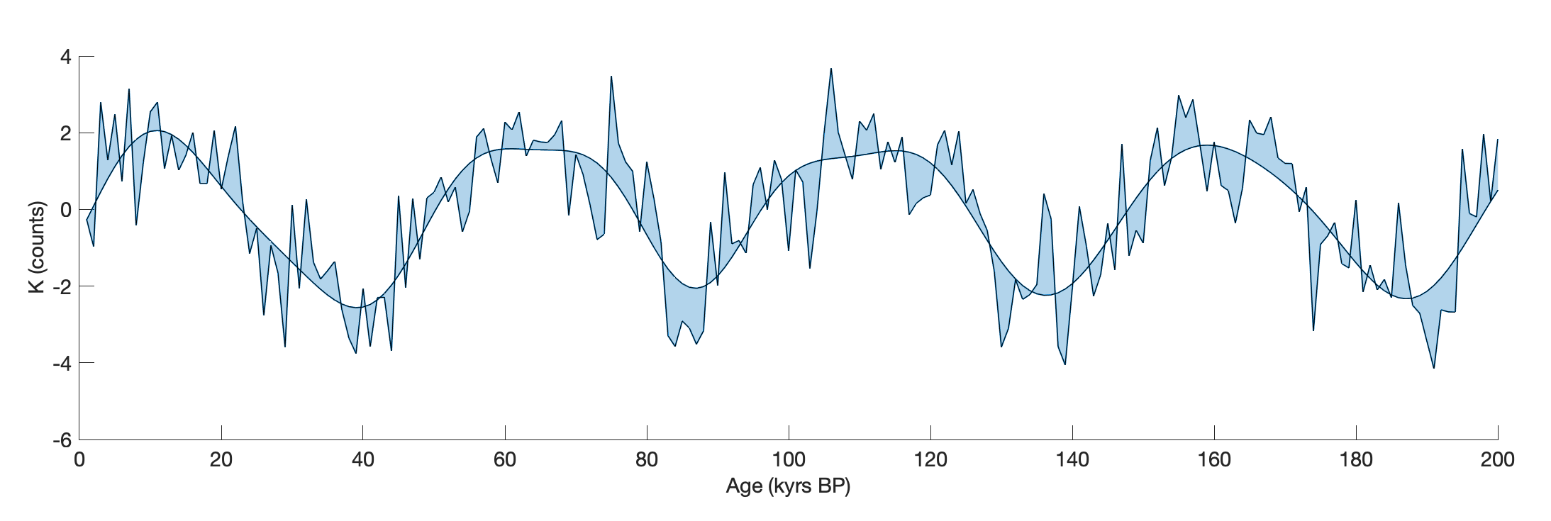
We can then display the two curves together with a filled polygon between the two using patch.
figure('Position',[1250 400 1200 400],...
  'Color',[1 1 1])
axes('Position',[0.1 0.2 0.8 0.65],...
  'XLim',[0 200],...
  'FontSize',14); hold on
line(t,x,...
  'LineWidth',1)
line(t,xf,...
  'LineWidth',1)
patch(tt,xxf,[0 114 189]/256,...
  'FaceAlpha',0.3)
xlabel('Age (kyrs BP)',...
  'FontSize',14)
ylabel('K (counts)',...
  'FontSize',14)