Convolving distributions corresponds to adding independent random variables. MATLAB is a great tool to demonstrate the convolution of distributions.
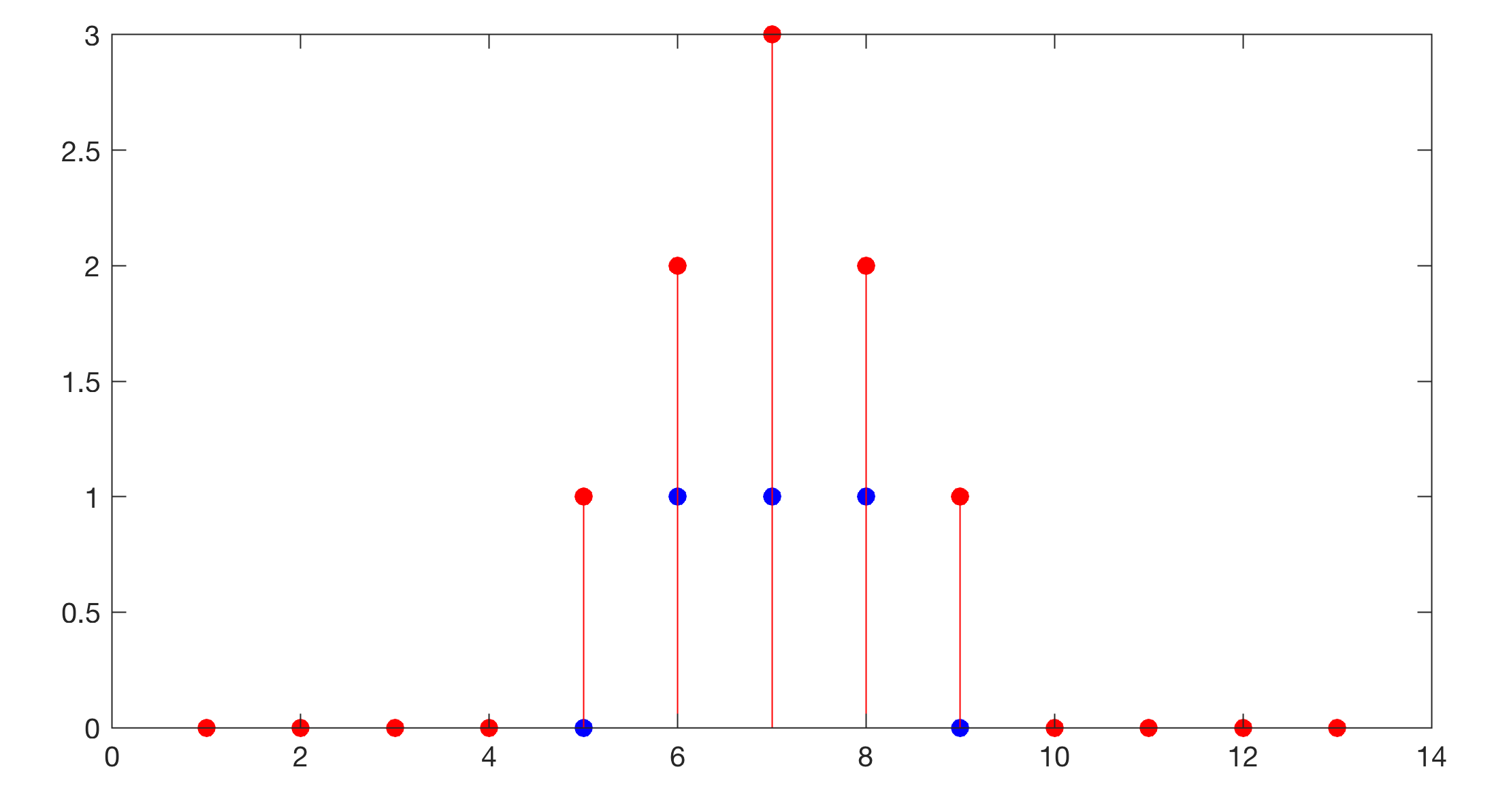
First we run an example of convolving two rect functions with MATLAB. Using the option same with conv(A,B) returns the central part of the convolution that is the same size as A.
clear
x = 1 : 13;
y1 = [0 0 0 0 0 1 1 1 0 0 0 0 0];
y2 = [0 0 0 0 0 1 1 1 0 0 0 0 0];
yc = conv(y1,y2,'same');

figure1 = figure('Color',[1 1 1],...
   'Position',[50 1000 600 300]);
stem(x,y1), hold on
stem(x,y2,'b','filled')
stem(x,yc,'r','filled')
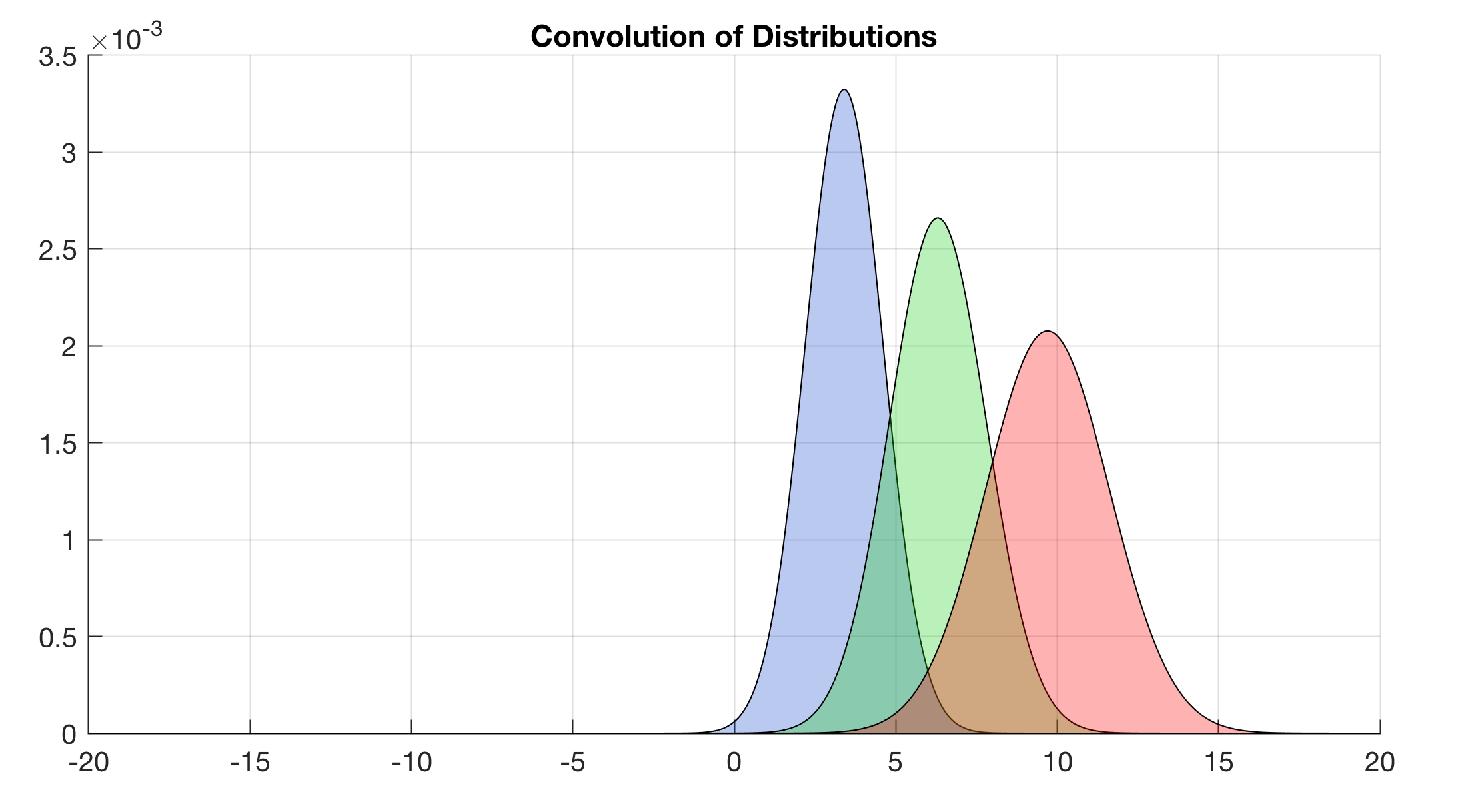
Next we convolve two Gaussian distributions. The convolution of the distributions yields an new Gaussian distribution with the mean of the sum of the separate means 3.4+6.3 = 9.7. We use patch with alpha(0.3) to display the result.
clear
agemean1 = 3.4; agestd1 = 1.2;
agemean2 = 6.3; agestd2 = 1.5;

x = -20: 0.01 : 20; x = x';
y1 = normpdf(x,agemean1,agestd1);
y1 = y1 ./ sum(y1);
maxx1 = x(y1==max(y1))
y2 = normpdf(x,agemean2,agestd2);
y2 = y2 ./ sum(y2);
maxx2 = x(y2==max(y2))

xc = 2*x;
yc = conv(y1,y2)*(x(2)-x(1));
yc = interp1(xc,yc(1:2:end),x,...
   'linear','extrap');
yc = yc./sum(yc);
maxxc = x(yc==max(yc))

figure2 = figure('Color',[1 1 1],...
   'Position',[50 600 600 300]);
patch(x,y1,[0.1 0.3 0.8]), hold on
patch(x,y2,[0.1 0.8 0.1])
patch(x,yc,[1 0 0])
alpha(0.3)
title('Convolution of Distributions')
grid, hold off
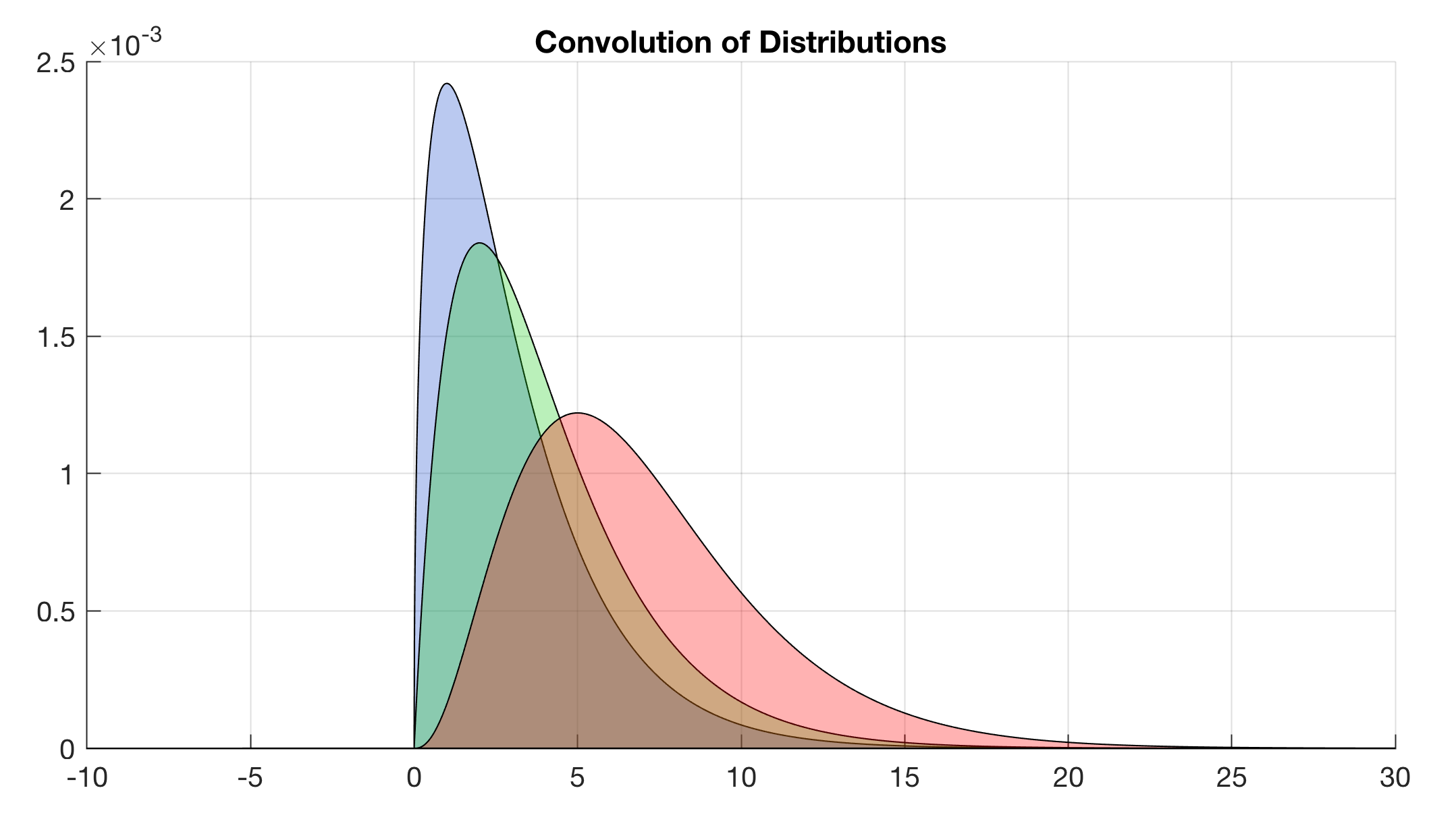
Then we try the same experiment with two Gamma distributions. If the scale b of gamma(p,b) is the same then the convolution of the Gamma distributions is also a Gamma distribution with gamma(p1+p2,b). The result y3 seems to be correct and what is expected. In our example the shape factors are 1.5 and 2 while the scale factor is always 2. Then we get another Gamma distribution with a shape factor of 1.5+2 = 3.5. The modes are 1, 2 and 5, whereas the expected values are 0.75, 1 and 1.75 (the sum).
clear
x = -10 : 0.01 : 30; x = x';
y1 = gampdf(x,1.5,2);
y1 = y1 ./ sum(y1);
maxx1 = x(y1==max(y1)),expx1 = 1.5/2
y2 = gampdf(x,2.0,2);
y2 = y2 ./ sum(y2);
maxx2 = x(y2==max(y2)),expx2 = 2/2
y3 = gampdf(x,1.5+2,2);
y3 = y3 ./ sum(y3);
maxx3 = x(y3==max(y3)),expx3 = (1.5+2)/2

xc = 2*x;
yc = conv(y1,y2)*(x(2)-x(1));
yc = interp1(xc,yc(1:2:end),x,...
'linear','extrap'); xc = x;
yc = yc./sum(yc);
maxxc = x(yc==max(yc))

figure2 = figure('Color',[1 1 1],...
   'Position',[50 200 600 300]);
patch(x,y1,[0.1 0.3 0.8]), hold on
patch(x,y2,[0.1 0.8 0.1])
patch(x,yc,[1 0 0])
alpha(0.3)
title('Convolution of Distributions')
grid, hold off