During our current summer school on Earth Surface Dynamics 2018 we learned how to calculate the Normalized Difference Vegetation Index (NDVI) from Sentinel-2 images. Here is a simple MATLAB script to import Sentinel-2 images and to calculate the NDVI.
Sentinel-2 is a system of four satellites built to perform terrestrial observations including forest monitoring, mapping land surface changes and natural desasters. The data can be downloaded free of charge at the USGS EarthExplorer after creating a user account. We use to images, acquired on 22 and 29 May 2018, from which we load the 650 nm (B04) and 850 nm (B08) spectral bands required to calculate the NDVI.
clear, clc, close all
filename1 = 'T32UQD_20180522T102031_B04_10m.jp2';
filename2 = 'T32UQD_20180522T102031_B08_10m.jp2';
filename3 = 'T32UQD_20180529T101031_B04_10m.jp2';
filename4 = 'T32UQD_20180529T101031_B08_10m.jp2';
B04_22 = imread(filename1);
B08_22 = imread(filename2);
B04_29 = imread(filename3);
B08_29 = imread(filename4);
We clip the image of the Berlin-Brandenburg area to the area of the city of Potsdam by typing
clip = [8500 9500 6500 7500];
B04_22 = B04_22(8500:9500,6500:7500);
B08_22 = B08_22(clip(1):clip(2),clip(3):clip(4));
B04_29 = B04_29(clip(1):clip(2),clip(3):clip(4));
B08_29 = B08_29(clip(1):clip(2),clip(3):clip(4));
Next we convert the uint16 data to single precision for calculations.
B04_22 = single(B04_22);
B08_22 = single(B08_22);
B04_29 = single(B04_29);
B08_29 = single(B08_29);
For display of the images we calculate the 5% and 95% percentiles.
B04_22_05 = prctile(reshape(B04_22,1,...
   numel(B04_22)), 5);
B04_22_95 = prctile(reshape(B04_22,1,...
   numel(B04_22)),95);
B08_22_05 = prctile(reshape(B08_22,1,...
   numel(B08_22)), 5);
B08_22_95 = prctile(reshape(B08_22,1,...
   numel(B08_22)),95);
B04_29_05 = prctile(reshape(B04_29,1,...
   numel(B04_29)), 5);
B04_29_95 = prctile(reshape(B04_29,1,...
   numel(B04_29)),95);
B08_29_05 = prctile(reshape(B08_29,1,...
   numel(B08_29)), 5);
B08_29_95 = prctile(reshape(B08_29,1,...
   numel(B08_29)),95);
Then we calculate the NDVI of both images by typing
NDVI_22 = (B08_22-B04_22)./(B08_22+B04_22);
NDVI_29 = (B08_29-B04_29)./(B08_29+B04_29);
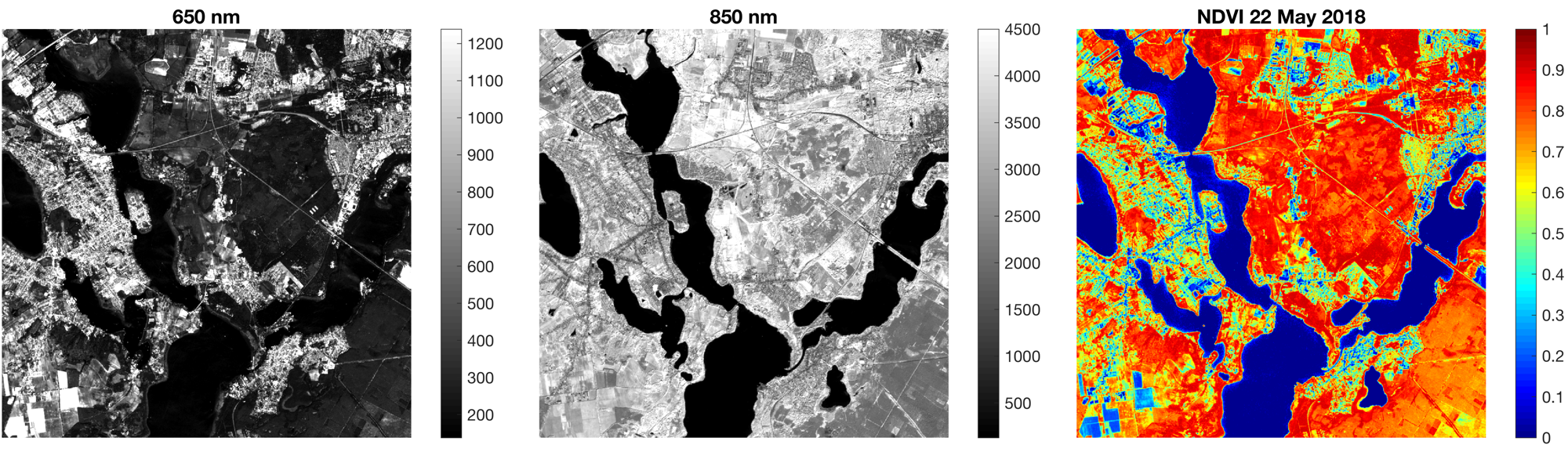
As an example we display the 650 nm and 850 nm spectral bands of the image acquire on 22 May 2018 as grayscale images and the NDVI map as color image using the colormap jet
figure('Position',[100 100 1400 400])
A1 = axes('Position',[0.025 0.1 0.4 0.8]);
imagesc(B04_22,[B04_22_05 B04_22_95])
title('650 nm')
colormap(A1,'Gray'), colorbar
set(gca,'FontSize',14)
axis square tight, axis off
A2 = axes('Position',[0.325 0.1 0.4 0.8]);
imagesc(B08_22,[B08_22_05 B08_22_95])
title('850 nm')
colormap(A2,'Gray'), colorbar
set(gca,'FontSize',14)
axis square tight, axis off
A3 = axes('Position',[0.625 0.1 0.4 0.8]);
imagesc(NDVI_22,[0 1])
title('NDVI 22 May 2018')
colormap(A3,'Jet'), colorbar
set(gca,'FontSize',14)
axis square tight, axis off
and save the image in a PNG file.
print -dpng -r300 sentinel_ndiv_1_vs1.png
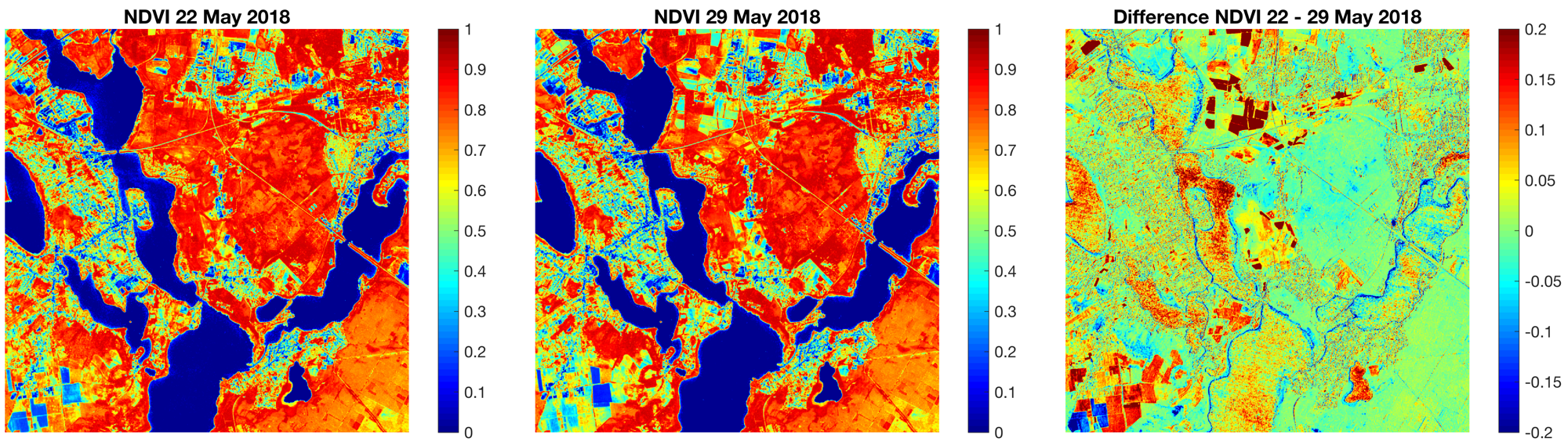
Then we calculate the difference between the NDVI maps of the two images aquired on 22 and 29 May 2018 to display the progress in the seasonal greening and again save the image in a PNG file.
DNDVI = NDVI_22 - NDVI_29;
figure('Position',[100 800 1400 400])
A3 = axes('Position',[0.025 0.1 0.4 0.8]);
imagesc(NDVI_22,[0 1])
title('NDVI 22 May 2018')
colorbar, set(gca,'FontSize',14)
colormap(A3,jet)
axis square tight, axis off
A4 = axes('Position',[0.325 0.1 0.4 0.8]);
imagesc(NDVI_29,[0 1])
title('NDVI 29 May 2018')
colorbar, set(gca,'FontSize',14)
colormap(A4,jet)
axis square tight, axis off
A5 = axes('Position',[0.625 0.1 0.4 0.8]);
imagesc(DNDVI,[-0.2 0.2])
title('Difference NDVI 22 - 29 May 2018')
colormap(A5,'Jet'), colorbar
set(gca,'FontSize',14)
axis square tight, axis off

print -dpng -r300 sentinel_ndiv_2_vs1.png