Colormaps are a graphical representation of data values as colors. MATLAB has a number of builtin colormaps. If you are tired of these there are several options to create and use alternative colormaps.
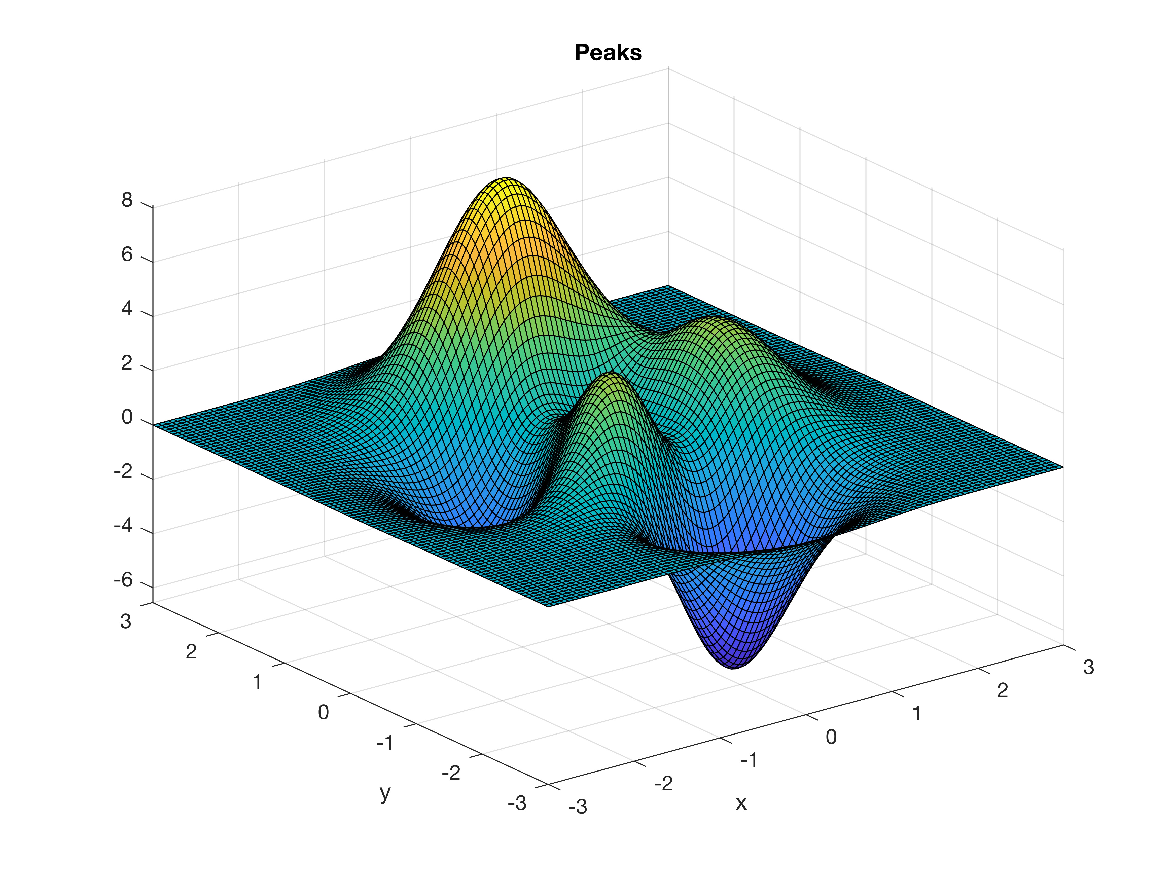
Typing help colormap opens the MATLAB docs and displays the help of the colormap function. There you will find the classic peaks example, a sample function of two variables. Typing
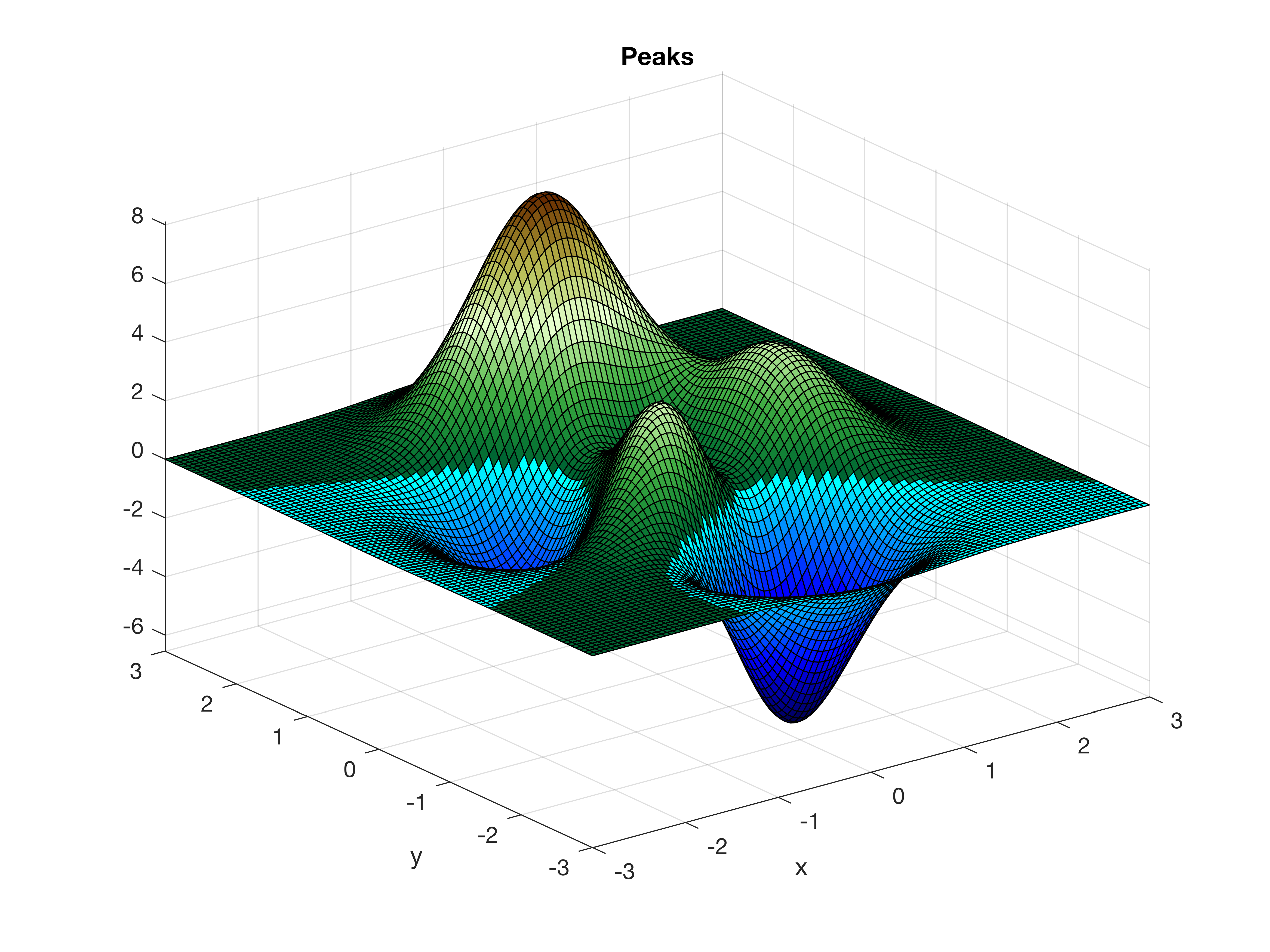
figure
peaks(100)
yields
z = 3*(1-x).^2.*exp(-(x.^2) - (y+1).^2) ...
    - 10*(x/5 - x.^3 - y.^5).*exp(-x.^2-y.^2) ...
    - 1/3*exp(-(x+1).^2 - y.^2)
and creates a three-dimensional surface using the standard colormap parula (see an earlier post Exporting EPS Files from MATLAB with CMYK Colors about colors and parula).
Typing
help graph3d
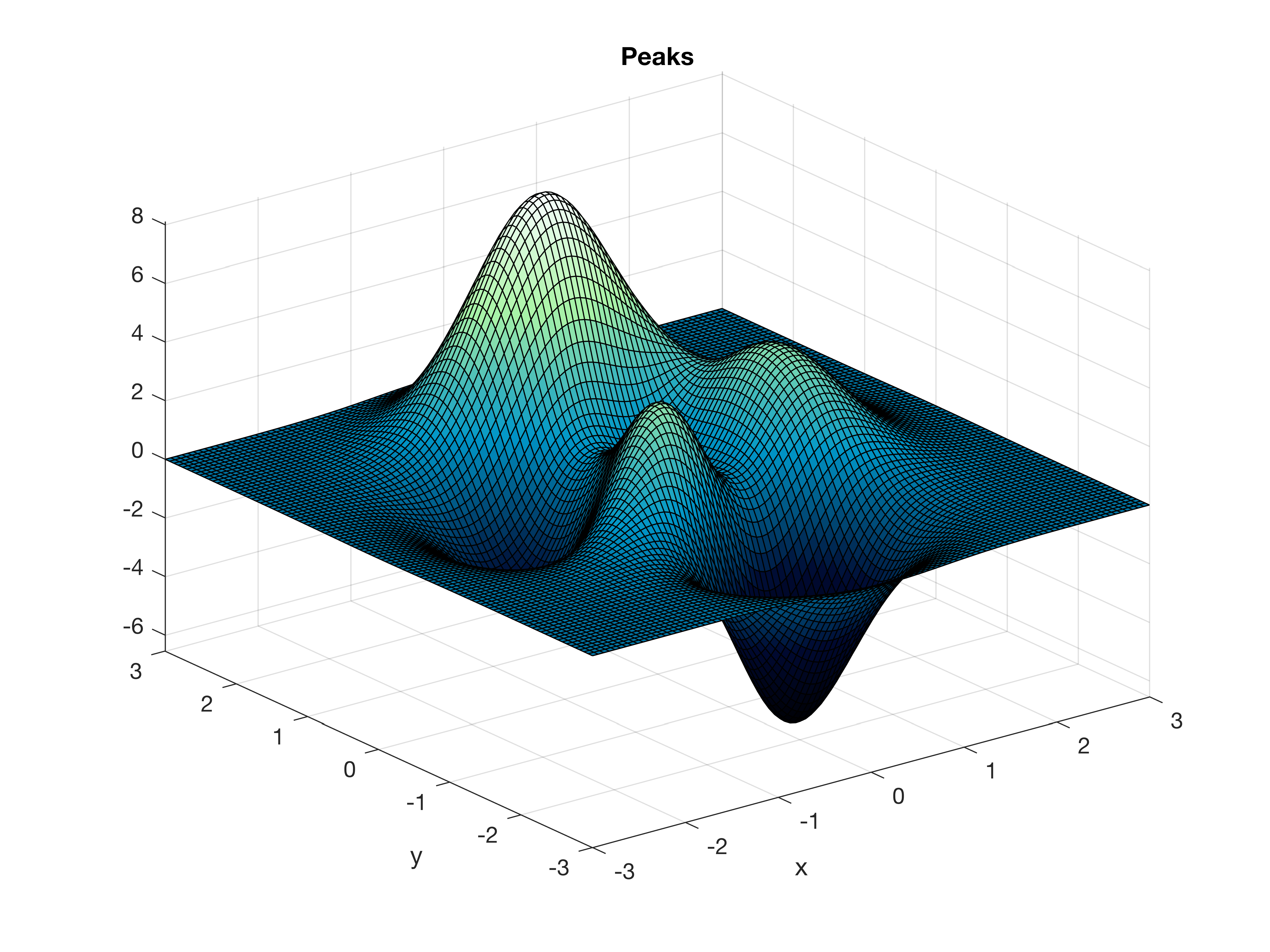
yields a list of the available builtin colormaps. We can change the colormap by typing
figure
peaks(100)
colormap(winter)
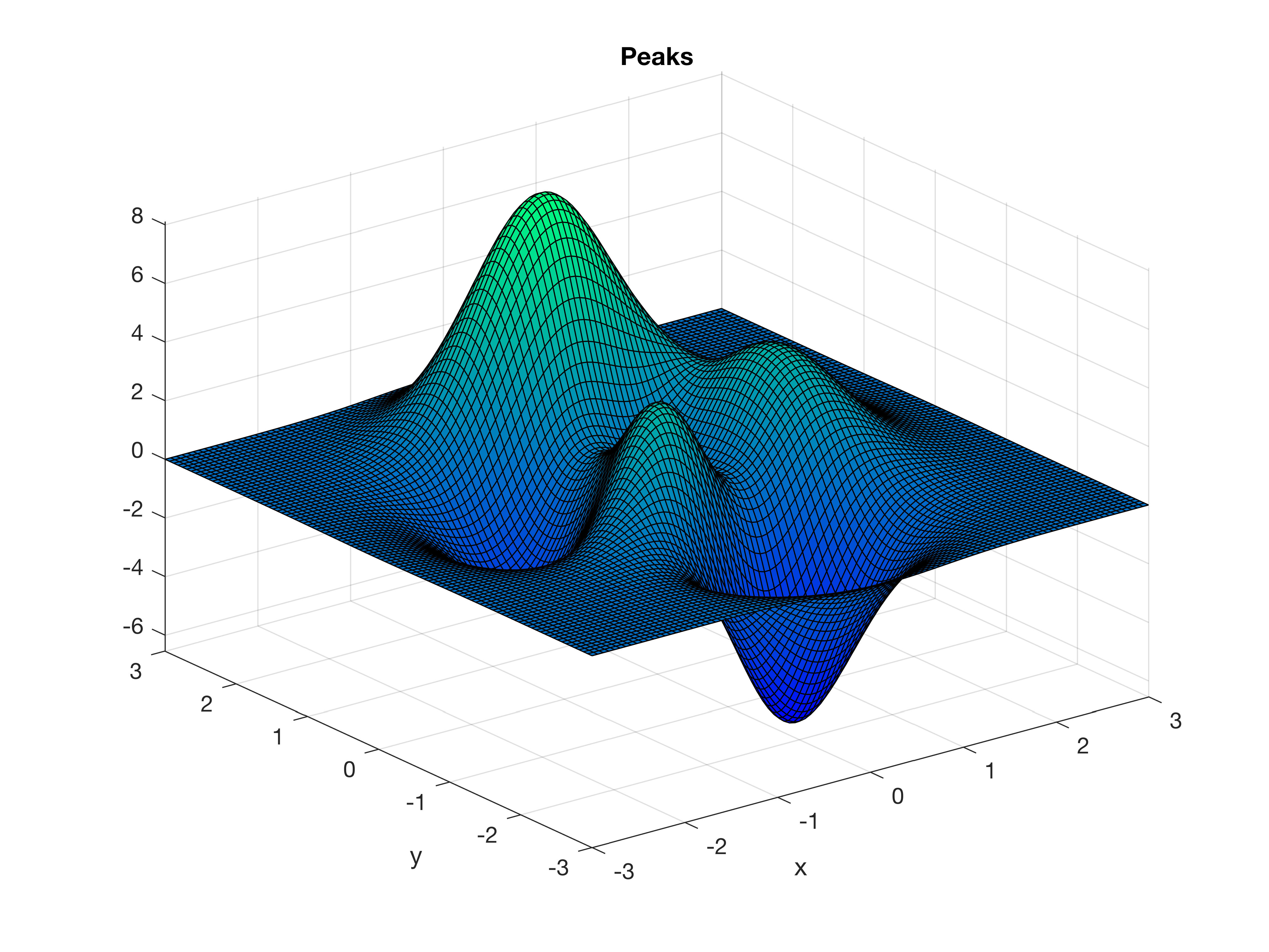
They are three-column arrays containing red, green, blue (RGB) triplets with values between 0 and 1 in which each row defines a specific color. You can easily create your own colormap, for instance, by designing a function which calculates such RGB triplets. As an example the colormap precip.m (which is a yellow-blue colormap included in MRES file collection) was created to display precipitation data, with yellow representing low rainfall and blue representing high rainfall. By default, low values are display in blue and high values in yellow, therefore we flip the colormap up and down to display high precipitation values in blue color.
figure
peaks(100)
colormap(flipud(precip))
For topographic data we can use the function demcmap contained in the Mapping Toolbox.
figure
peaks(100)
demcmap(peaks(100))
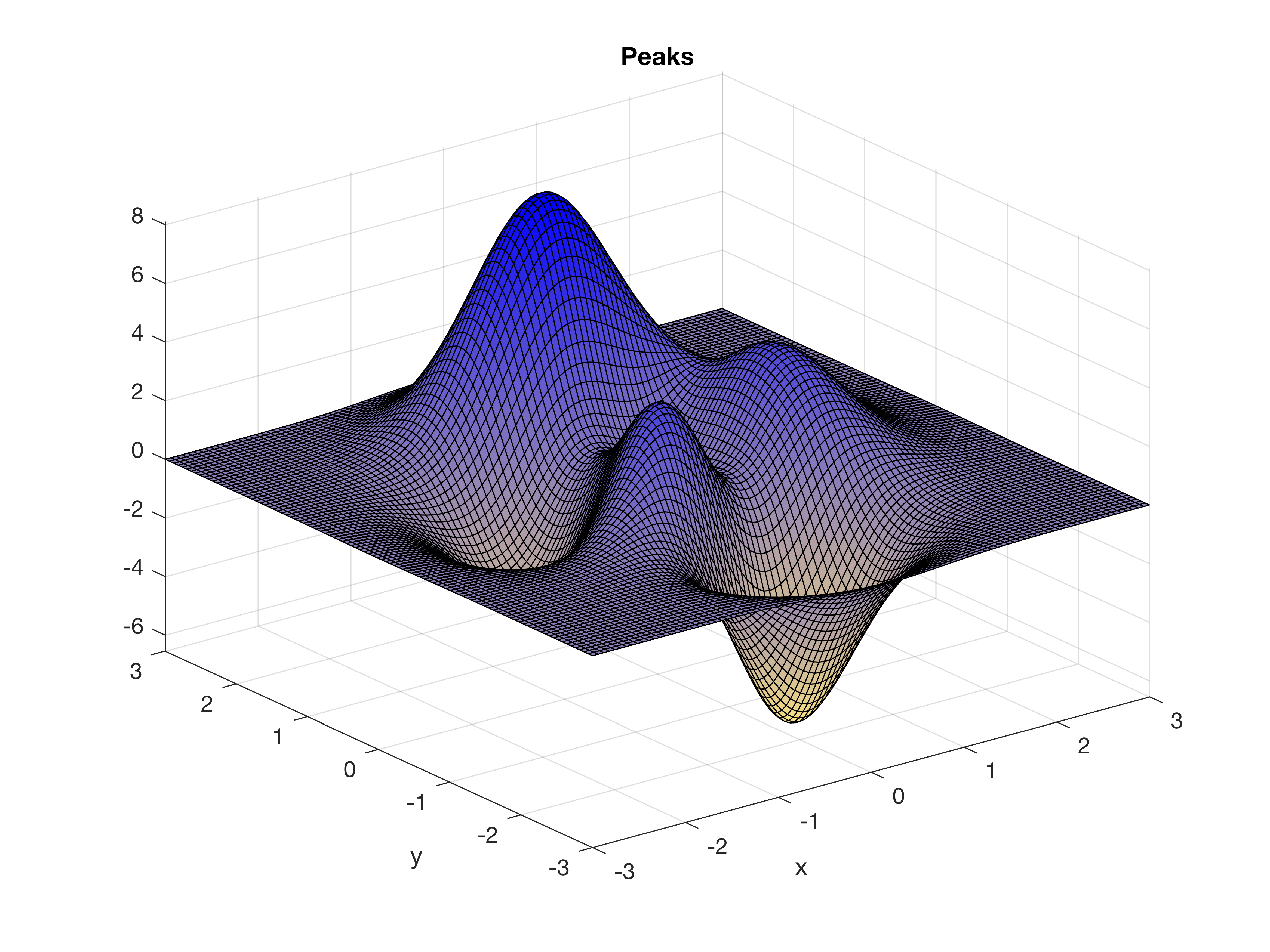
If you do not need the Mapping Toolbox there are excellent free alternatives to the demcmap colormap. My favorite toolbox is the cptcmap of Kelly Kearney available online at the MATLAB file exchange. The toolbox contains a number of useful colormaps, mostly to display earth science data. As an example we can use the GMT_ocean colormap by typing
figure
peaks(100)
cptcmap('GMT_ocean')