In a series of blog posts, I will tell you a little about how I teach computational geosciences with MATLAB. On the second half of day 4 of the one-week course I teach to import, process, analyze and visualize spatial data.
After three days with lessons on statistical methods, in particular time series analysis, participants on the fourth day very much appreciate the analysis of spatial data. This part of the course is far less demanding, requires little mathematical basic knowledge and includes beautiful 3D graphics.
We start with vector graphics, such as the Global Geography Database (GSHHG) data set consisting of world shorelines. Then we continue with the ETOPO1 data set, the SRTM data set and finish with 3D animations. Creating animated 3D files with MATLAB for inclusion in documents such as multimedia ebooks, interactive webpages, and presentations was recently discussed in the June 2017 issue of the MATLAB Digest | Academic Edition by Lisa Webb. The method is used while creating the interactive edition of MRES.
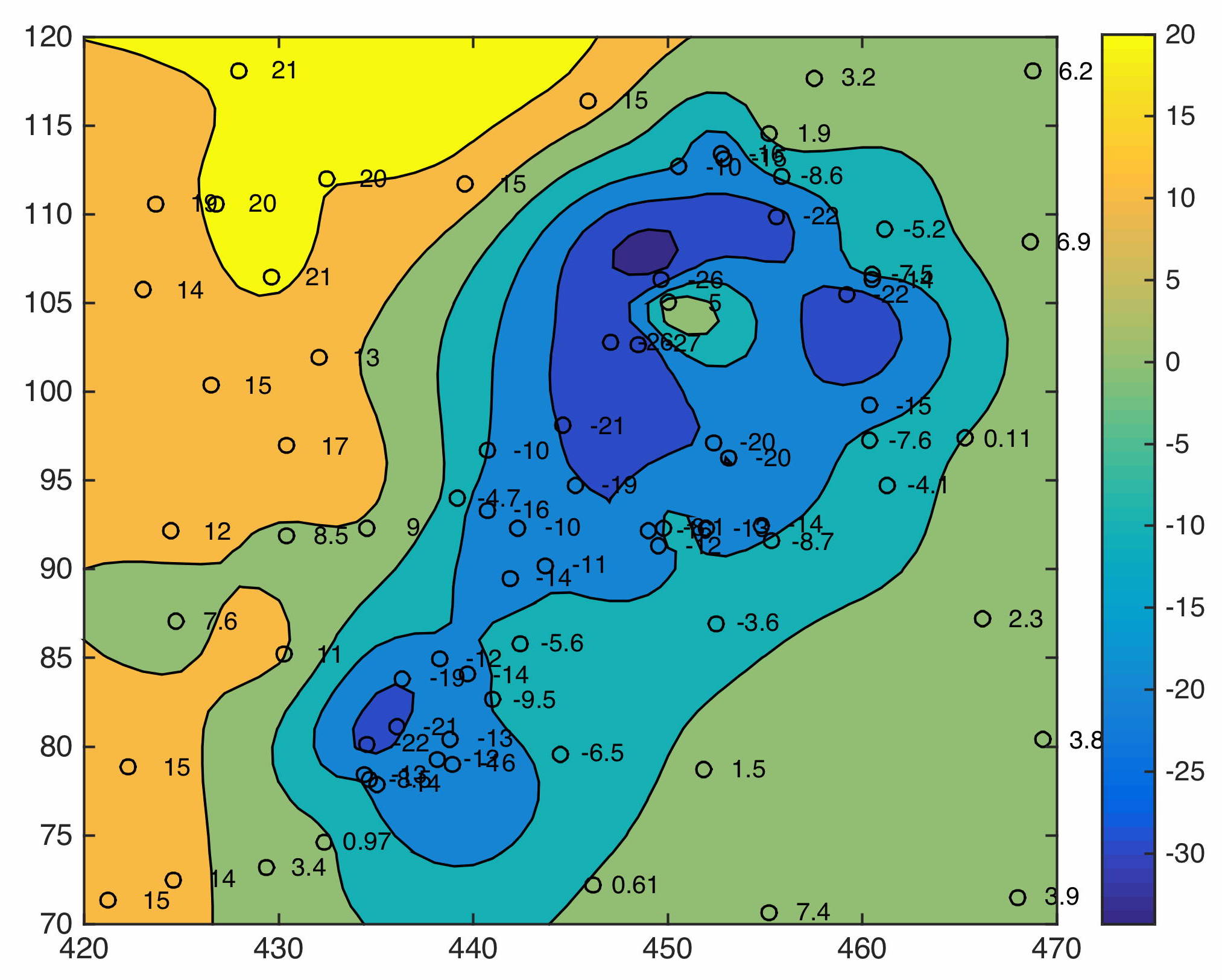
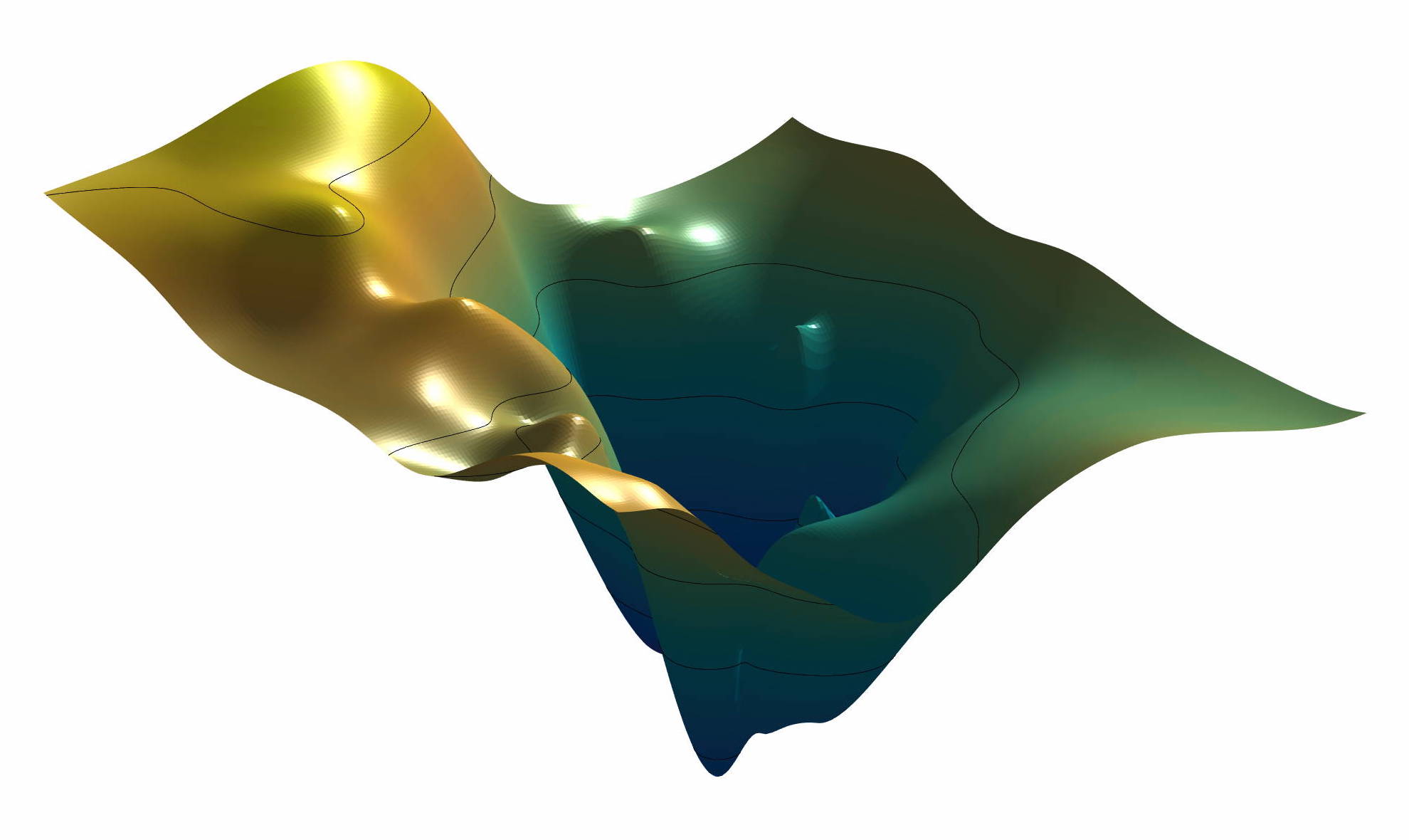
The somewhat more demanding part of the course on spatial data presents interpolation methods, such as linear interpolation, cubic and biharmonic splines. Here, special attention is paid to possible artifacts in the wrong use of the methods. Unfortunately, the literature is full of such erroneous interpolation results, so it is important to me to draw my students’ attention to possible problems.