
In a series of blog posts, I will tell you a little about how I teach computational geosciences with MATLAB. On the second half of day 3 of the one-week course I teach signal processing.
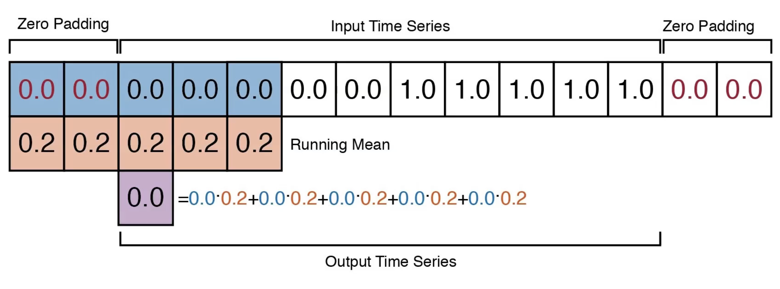
First, I explain the principle of convolution. We use a running mean of a length of five in MATLAB to smooth a time series of random numbers. In this case, it is already noticeable that the smoothed signal shows clear reversals of the amplitudes in a particular wavelength range. As said in an earlier post about why better avoid running means we can use the frequency characteristics of the filter to explain why some frequencies disappear and some are reversed.
The better solution for smoothing signals are low-pass filters. I explain the design of filters using the Butterworth approach, but this requires an arbitrary choice of cutoff frequencies. For this reason, we complete the teaching of signal processing with adaptive filters, which automatically extract the signal from a noisy signal (see an earlier post about adaptive filters). The course day with sophisticated examples from the frequency domain ends with this and we continue the course the next day with multivariate statistics and digital terrain models.