
In a series of blog posts, I will tell you a little about how I teach computational geosciences with MATLAB. After the work environment is set up and resources are presented with information about MATLAB, I show a very simple example of the typical workflow with MATLAB. The main goal of this is to show beginners how easy it is to get into this huge software.
After the installation of MATLAB, the software is launched either by clicking the shortcut icon on the desktop or by typing
matlab
in the operating system prompt. The software then comes up with several window panels. The default desktop layout includes the Current Folder panel that lists the files in the directory currently being used. The Command Window presents the interface between the software and the user, i.e., it accepts MATLAB commands typed after the prompt, >>. The Workspace panel lists the variables in the MATLAB workspace, which is empty when starting a new software session. In this book we mainly use the Command Window and the built-in Editor, which can be launched by typing
edit
By default, the software stores all of your MATLAB-related files in the startup folder named MATLAB. Alternatively, you can create a personal working directory in which to store your MATLAB-related files. You should then make this new directory the working directory using the Current Folder panel or the Folder Browser at the top of the MATLAB desktop. The software uses a Search Path to find MATLAB-related files, which are organized in directories on the hard disk. The default search path includes only the directory that has been created by the installer in the applications folder and the default working directory MATLAB.
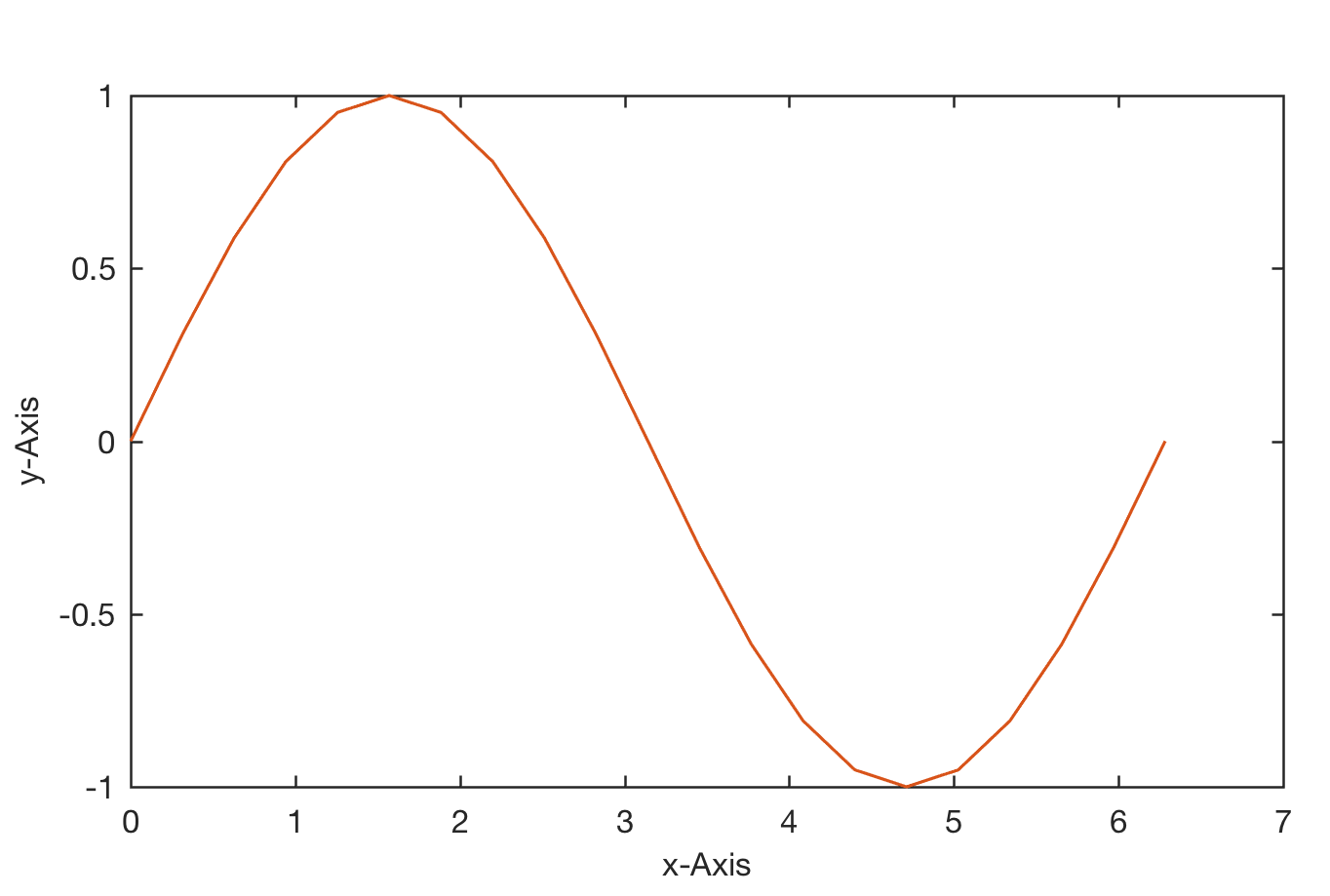
As an example, we create two one-dimensional arrays x and y, where y is the sine of x. The array x contains values between 0 and 2π with π/10 increments, whereas y is the element-by-element sine of x.
x = 0 : pi/10 : 2*pi;
y1 = sin(x);
These two commands result in two one-dimensional arrays with 21 elements each, i.e., two 1-by-21 arrays. Since the two arrays x and y have the same length, we can use plot to produce a linear 2D graph of y against x.
plot(x,y1)
This command opens a Figure Window named Figure 1 with a gray background, an x-axis ranging from 0 to 7, a y-axis ranging from –1 to +1 and a blue line. This is it – with the exception of importing some data, which is shown later, we have a calculation and a subsequent graphical display of the results. It will then be shown how the graphics can be saved and printed. In addition, the Publishing feature and the Live Editor is shown, with which one can create sophisticated reports. On the afternoon of the first day, advanced graphics are shown, which can be used to create a graphic that can be published from the data generated above.
x = 0 : pi/10 : 2*pi;
y1 = sin(x);

figure1 = figure(...
    'Position',[200 200 800 600],...
    'Color',[1 1 1]);
axes1 = axes(...
    'Box','on',...
    'Units','Centimeters',...
    'Position',[2 2 10 6],...
    'LineWidth',0.6,...
    'FontName','Helvetica',...
    'FontSize',8);
line(x,y1,...
    'LineWidth',0.75,...
    'Color',[0.8477 0.3242 0.0977]);
xlabel(...
 'x-Axis',...
 'FontName','Helvetica',...
 'FontSize',8);
ylabel(...
 'y-Axis',...
 'FontName','Helvetica',...
 'FontSize',8);

print -dpng -r300 example_vs1.png
During the rest of the day I teach a standard introduction to the MATLAB syntax, data structures and classes of objects, data storage and handling, basic visualization tools and generating code to recreate graphics. Programming with MATLAB is taught during the MATLAB/LEGO MINDSTORMS practical.