Importing, Processing and Exporting LANDSAT Images with MATLAB – MATLAB and Python Recipes for Earth Sciences

MATLAB is now a widely used tool in satellite remote sensing. Here is an example of importing, processing, and exporting freely-available Landsat images of Lake Naivasha in the Central Kenya Rift.

The Landsat project is a satellite remote sensing program jointly managed by the US National Aeronautics and Space Administration (NASA) and the US Geological Survey (USGS), which began with the launch of the Landsat 1 satellite (originally known as the Earth Resources Technology Satellite 1) on 23rd July 1972. The latest in a series of successors is the Landsat 8 satellite, launched on 11th February 2013 (Ochs et al. 2009, Irons et al. 2011). It has two sensors, the Operational Land Imager (OLI) and the Thermal Infrared Sensor (TIRS). These two sensors provide coverage of the global landmass at spatial resolutions of 30 meters (visible, NIR, SWIR), 100 meters (thermal), and 15 meters (panchromatic) (Ochs et al. 2009, Irons et al. 2011).

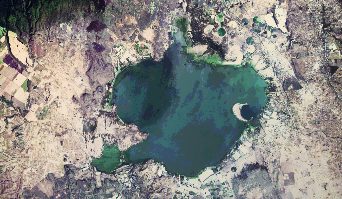
General information concerning the Landsat program can be obtained from the Landsat webpage at NASA. Landsat data, together with data from other NASA satellites, can be obtained from the USGS EarthExplorer webpage. As example we find an image of the Central Kenya Rift dated 17 January 2017. We can import the 118.4 MB TIFF files for the channels B4, B3 and B2 using

clear, close all, clc
filename = ...
    'LC08_L1TP_169060_20170117_20170311_01_T1_';
channels = ['B4';'B3';'B2'];
extension = '.TIF';
I1 = imread([filename,channels(1,:),extension]);
I2 = imread([filename,channels(2,:),extension]);
I3 = imread([filename,channels(3,:),extension]);

Since the image has a relatively low level of contrast, we use adapthisteq to perform a contrast-limited adaptive histogram equalization. Then the three bands are concatenated to a 24-bit RGB images using cat.

I1 = adapthisteq(I1,'ClipLimit',0.1);
I2 = adapthisteq(I2,'ClipLimit',0.1);
I3 = adapthisteq(I3,'ClipLimit',0.1);
I = cat(3,I1,I2,I3);

We only display that section of the image containing Lake Naivasha (using axes limits) and hide the coordinate axes. We scale the images to 20% of the original size to fit the computer screen. Exporting the processed image from the Figure Window, we only save the image at the monitor’s resolution. To obtain an image of the basins at a higher resolution, we use the command imwrite.

figure('Position',[100 100 800 800])
axes('XLim',[5000 6200],...
     'YLim',[6300 7000],...
     'Visible','Off'), hold on
imshow(I,'InitialMagnification',20)
imwrite(I(6300:7000,5000:6200,:),...
     'naivasha.png','png')

References

Irons J, Riebeek H, Loveland T (2011) Landsat Data Continuity Mission – Continuously Observing Your World. NASA and USGS (available online)

Ochs B., Hair D, Irons J, Loveland T (2009) Landsat Data Continuity Mission, NASA and USGS (available online)