
 Detecting change points, such as abrupt transitions in the mean, the variance, the trend in time series is an important task of modern time series analysis. As an example, possible tipping points in the Earth’s climate system are currently being intensively investigated. Detecting, not predicting, change points in time series can be done using various methods with MATLAB, including the function findchangepts introduced with release R2016a and contained in the Signal Processing Toolbox.
A number of methods are available to detect abrupt changes in time series in the time domain. The method I used in a paper about the statistical analysis of dust records (Trauth et al., 2009) was to assess differences in central tendency and dispersion between two different sliding windows. The method, together with the MATLAB script, is also described in Chapter 5.9 of MRES.
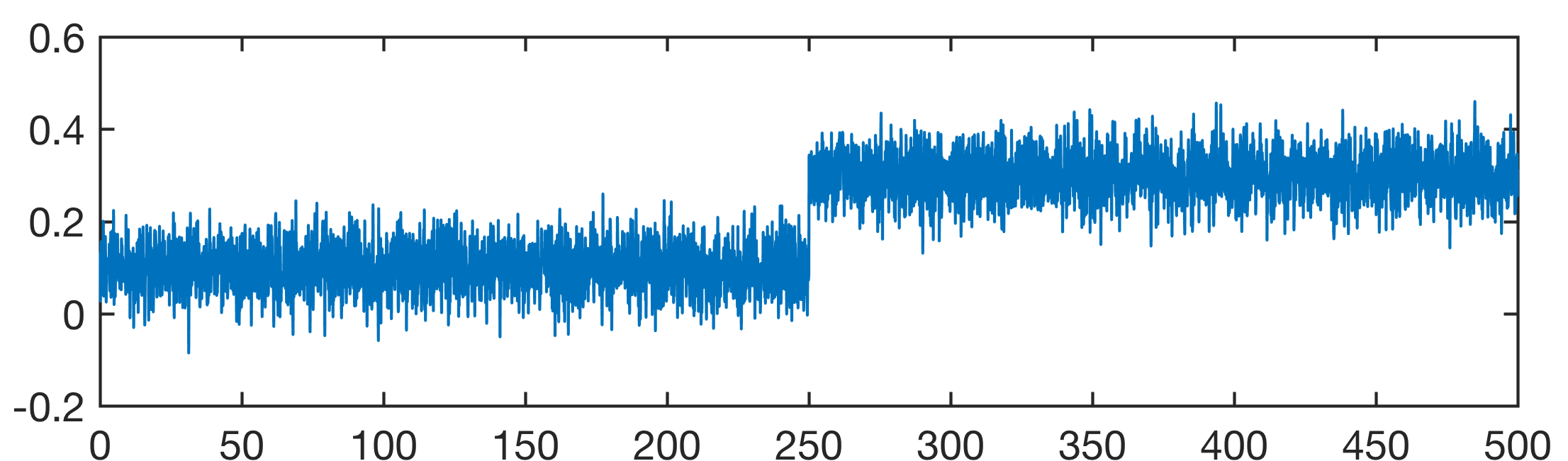
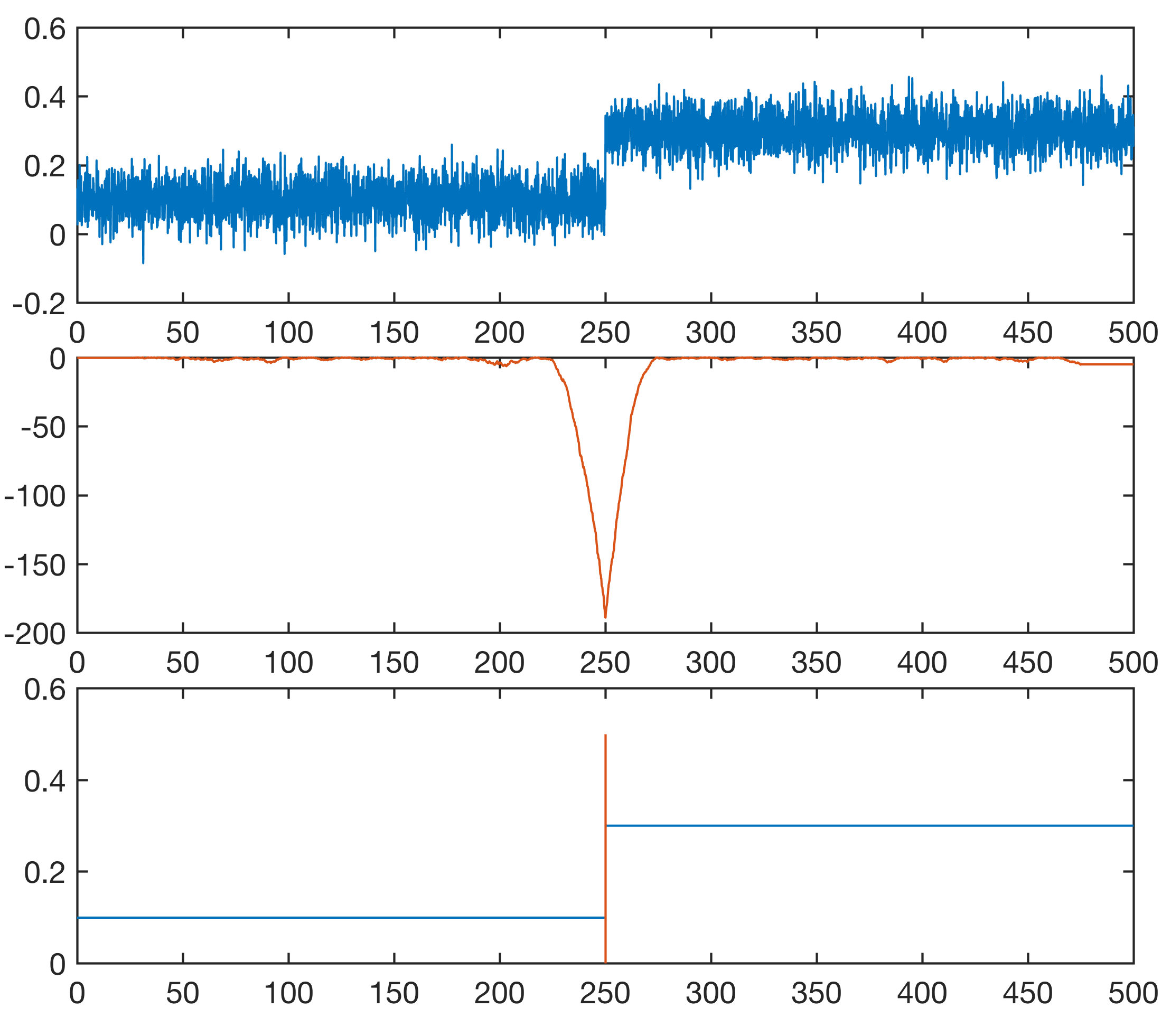
The example demonstrates the Mann-Whitney test on two synthetic records that contain a stepwise change of the mean at x=250.
clear
rng(10)
t = 0.1 : 0.1 : 500;
y1 = 0.1*random('norm',1,0.5,1,length(t),1);
y2 = 0.1*random('norm',3,0.5,1,length(t),1);
y = y1(1:length(t)/2);
y(length(t)/2+1:length(t)) = ...
    y2(length(t)/2+1:length(t));
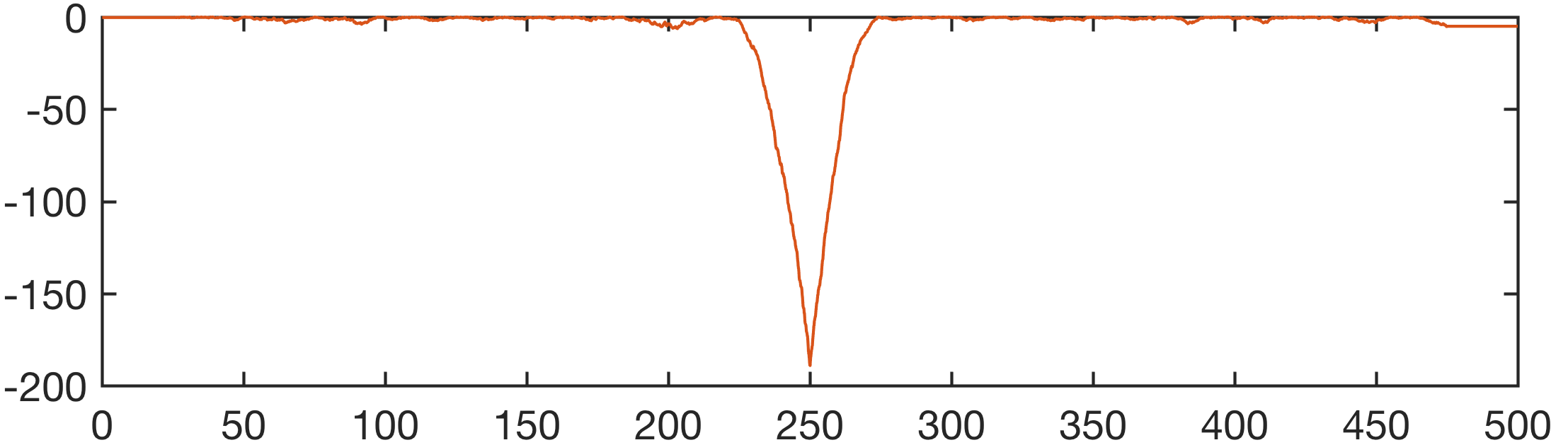
Then we use a Mann-Whitney test with paired sliding windows of the length of w = 500 data point, in order to detect any abrupt change in the mean. The first for loop can be used to use several windows of different length, such as w = [300 500 1000] instead of w = 500 only.
w = 500;
for j = 1:length(w)
na = w(j);
nb = w(j);
for i = w(j)/2+1:length(y)-w(j)/2
    [p,h] = ranksum(y(i-w(j)/2:i-1),...
    y(i+1:i+w(j)/2));
    mwreal(j,i) = p;
end
mwreal(j,1:w(j)/2) = ...
    mwreal(j,w(j)/2+1) * ones(1,w(j)/2);
mwreal(j,length(y)-w(j)/2+1:length(y)) = ...
mwreal(j,length(y)-w(j)/2) * ones(1,w(j)/2);
end
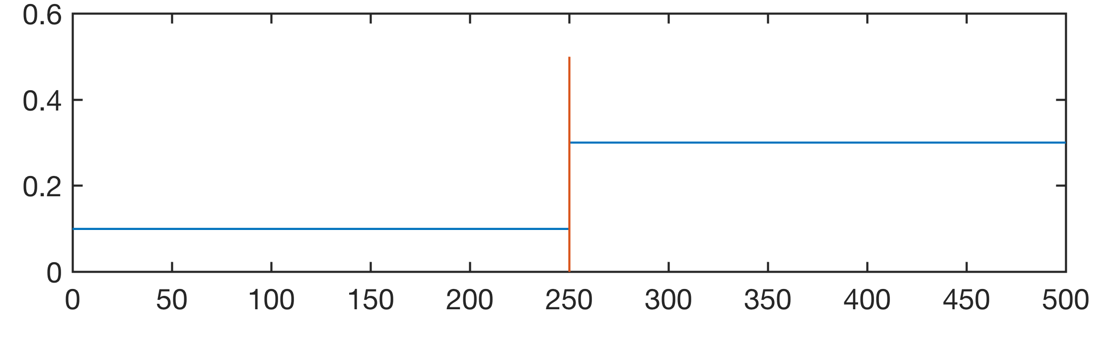
Alternatively we can use the new function findchangepts, which has recently been included in MATLAB to detect change points by minimising a cost function over all possible numbers and locations of change points. The function returns the largest number of significant changes in the mean, the standard deviation, and the trend of a time series, not exceeding a maximum number of permissible changes maxnumchg defined by the user, that minimize the sum of the residual error and an internal fixed penalty for each change.
maxnumchg = 1;
ipoint = findchangepts(y,...
    'Statistic','mean',...
    'MaxNumChanges',maxnumchg);
ipoint(end+1) = length(y);
m(1) = mean(y(1:ipoint(1)));
for i = 1 : length(ipoint)-1
    m(i+1) = mean(y(ipoint(i):ipoint(i+1)));
end
m(length(ipoint)+1) = mean(y(ipoint(i):end));
We can display the results in a single figure window:
figure('Position',[100 800 600 500],...
    'Color',[1 1 1]);
axes('Position',[0.1 0.7 0.8 0.25],...
    'Box','On',...
    'LineWidth',1,...
    'FontSize',14); hold on
line(t,y,...
    'LineWidth',1);
axes('Position',[0.1 0.4 0.8 0.25],...
    'Box','On',...
    'LineWidth',1,...
    'FontSize',14);
line(t,log(mwreal),...
    'LineWidth',1,...
    'Color',[0.8510 0.3255 0.0980]);
axes('Position',[0.1 0.1 0.8 0.25],...
    'XLim',[0 500],...
    'Box','On',...
    'LineWidth',1,...
    'FontSize',14); hold on
line([0 t(ipoint(1))],[m(1) m(1)],...
    'LineWidth',1)
for i = 1 : length(ipoint)-1
    line([t(ipoint(i)) t(ipoint(i+1))],...
    [m(i+1) m(i+1)],...
    'LineWidth',1)
end
line([t(ipoint(length(ipoint))) t(end)],...
    [m(end) m(end)],...
    'LineWidth',1)
stem(t(ipoint(1:end-1)),...
    0.5*ones(size(t(ipoint),2)-1),...
    'Marker','none',...
    'LineWidth',1,...
    'Color',[0.8510 0.3255 0.0980]);
References
Lavielle, M. (2005) Using penalized contrasts for the change-point problem. Signal Processing, 85, 1501–1510.
Killick, R., Fearnhead, P., Eckley, I.A. (2012) Optimal detection of changepoints with a linear computational cost. Journal of the American Statistical Association, 107, 1590–1598.
Schellnhuber, H.J. (2009) Tipping elements in the Earth System. PNAS, 106, 20561–20563.
Trauth MH, Larrasoaña JC, Mudelsee M (2009) Trends, rhythms and events in Plio-Pleistocene African climate. Quaternary Science Reviews, 28, 399–411