
Bioturbation (or benthic mixing) causes significant distortions in marine stable isotope signals and other palaeoceanographic records. In an earlier post I introduced a MATLAB-based model to study the effect of bioturbation on isotopic signals from stratigraphic carriers such as foraminifera. This post will demonstrate how to create a publishable figure showing the uppermost layers of a sediment sequence affected by bioturbation. The following posts will introduce MATLAB-based animations of the benthic mixing.
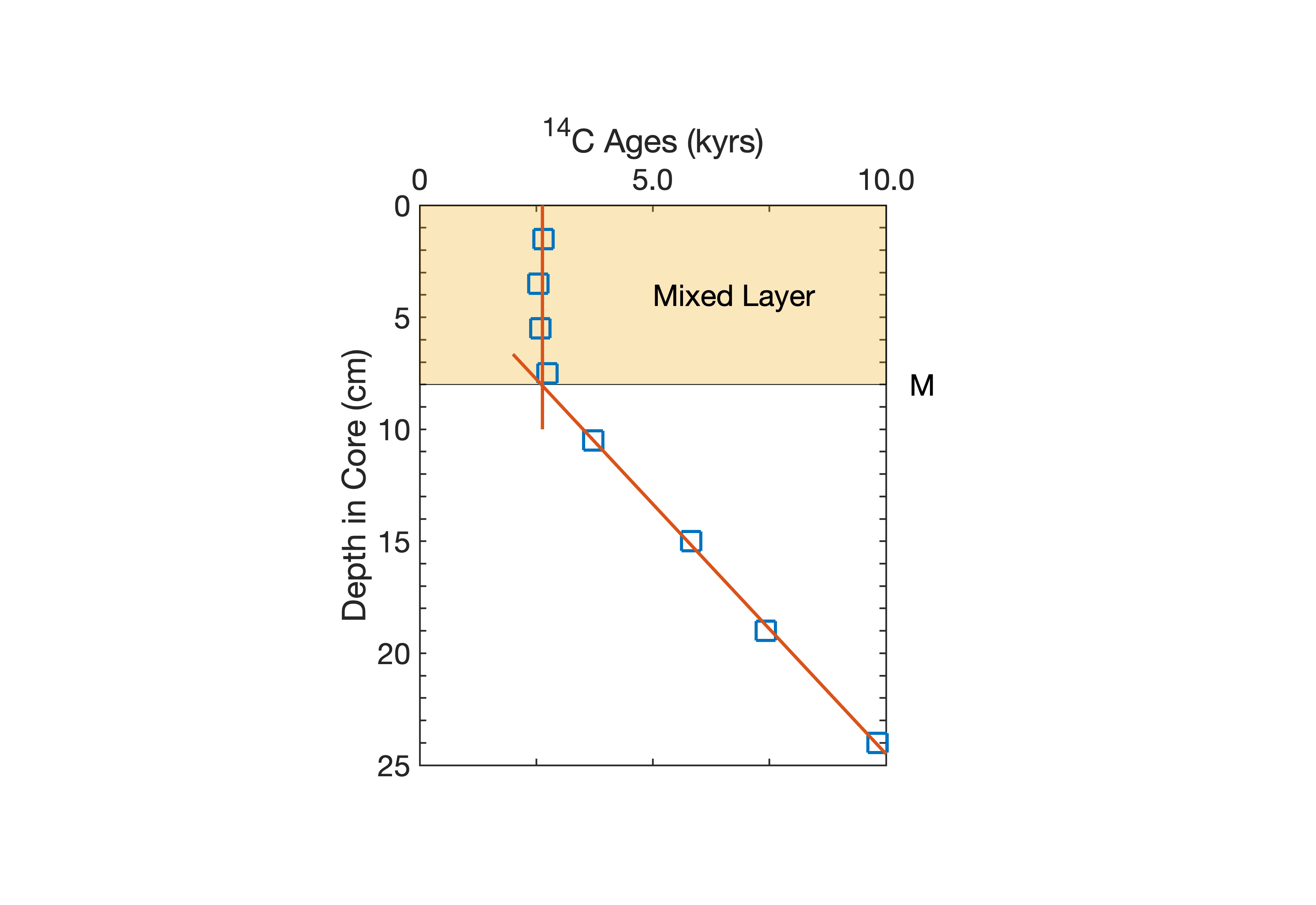
The classic way to describe benthic mixing or bioturbation on the deep-sea floor is to postulate a mixed layer of a specific thickness M (marked by yellow shading, typically between M=0 and M=20 cm, global average about M=8 cm), resting on top of a sediment pile that is not influenced by benthic activity (e.g. Berger and Heath, 1968). Many studies on the distribution of high-resolution 14C data series (marked by blue squares) in box core profiles have shown instantaneous mixing within such a layer and suggest that this model describes the process of bioturbation in the deep-sea sediments sufficiently accurately, at least on radiocarbon time scales. Here is a script to create a graphics similar to Figure 2 of my paper published in Paleoceanography (Trauth et al., 1997) which uses 14C data of Buffoni et al. (1992), showing the uppermost layers of a sediment sequence affected by bioturbation.
clc, clear, close all

data = [ 1.5 2.654
    3.5 2.546
    5.5 2.585
    7.5 2.743
   10.5 3.721
   15.0 5.821
   19.0 7.425
   24.0 9.820];

p1 = mean(data(1:4,2));
p2 = polyfit(data(5:end,2),data(5:end,1),1);

XTickLabelCell = {'0';' ';'5.0';' ';'10.0'};
YTickLabelCell = {'0';' ';' ';' ';' ';...
    '5';' ';' ';' ';' ';...
    '10';' ';' ';' ';' ';...
    '15';' ';' ';' ';' ';...
    '20';' ';' ';' ';' ';...
    '25'};

figure('Position',[50 100 800 550],...
    'Color',[1 1 1]);

axes('Units','Centimeters',...
    'Position',[9 3 10 12],...
    'XLim',[0 10],...
    'YLim',[0 25],...
    'Box','On',...
    'LineWidth',1,...
    'FontSize',18,...
    'XTickLabel',XTickLabelCell,...
    'XTick',[0 2.5 5.0 7.5 10.0],...
    'YTickLabel',YTickLabelCell,...
    'YTick',0:25,...
    'YDir','reverse',...
    'XAxisLocation','Top')

hold on

xlabel('^{14}C Ages (kyrs)')
ylabel('Depth in Core (cm)')

patch([0 10 10 0],[0 0 8 8],...
    [0.9290 0.6940 0.1250],...
    'FaceAlpha',0.3)

line(data(:,2),data(:,1),...
    'LineStyle','none',...
    'Marker','square',...
    'MarkerSize',15,...
    'LineWidth',2)
line([p1 p1],[0 10],...
    'Color',[0.8500 0.3250 0.0980],...
    'LineWidth',2)
line([2 10],polyval(p2,[2 10]),...
    'Color',[0.8500 0.3250 0.0980],...
    'LineWidth',2)

text(5,4,'Mixed Layer',...
    'FontSize',18)

text(10.5,8,'M',...
    'FontSize',18)

print -dpng -r300 bioturbationgraphics.png
References
Berger, W.H., Heath, R.G. (1968) Vertical mixing in pelagic sediments. Journal of Marine Research 26, 134–143.
Buffoni, G., Delfanti, R., Papucci, C. (1992): Accumulation rates and mixing processes in near-surface North Atlantik sediments: Evidence from C-14 and Pu-239,240 downcore profiles. – Mar. Geol., 109, 159-170.
Trauth, M.H., Sarnthein, M., Arnold, M. (1997) Bioturbational mixing depth and carbon flux at the seafloor. Paleoceanography, 12, 517-526.
Trauth, M.H. (1998) TURBO: a dynamic-probabilistic simulation to study the effects of bioturbation on paleoceanographic time series. Computers and Geosciences, 24(5), 433-441.
Trauth, M.H. (2013) TURBO2: A MATLAB simulation to study the effects of bioturbation on paleoceanographic time series. Computers and Geosciences, 61, 1-10.