
Principal component analysis (PCA) detects linear dependencies between variables and replaces groups of linear correlated variables with new, uncorrelated variables referred to as the principal components (PCs). The MATLAB function pca helps to perform such an linear unmixing experiment.
Principal component analysis (PCA) is the standard method for unmixing (or separating) mixed variables. PCA was introduced by Karl Pearson (1901) and further developed by Harold Hotelling (1931). Such analyses produce signals that are linearly uncorrelated, and this method is also called whitening since this property is characteristic of white noise. Although the separated signals are uncorrelated, they can still be interdependent, i.e., they may retain a nonlinear correlation. This phenomenon arises when, for example, the data are not Gaussian distributed and the PCA consequently does not yield good results. The independent component analysis (ICA) was developed for this type of task; it separates the variables X into independent variables S, which are then nonlinearly uncorrelated.
In the following example a synthetic data set is used to illustrate the use of the function pca included in the Statistics and Machine Learning Toolbox. Thirty samples were taken from thirty different levels in a sedimentary sequence containing varying proportions of the three different minerals stored in the columns of the array x. The sediments were derived from three distinct rock types (with unknown mineral compositions) whose relative contributions to each of the thirty sediment samples are represented by s1, s2 and s3. Variations in these relative contributions (as represented by the thirty values in s1, s2 and s3) could, for example, reflect climatic variability within the catchment area of the sedimentary basin. It may therefore be possible to use the sediment compositions in the array x (from which we calculate s1, s2 and s3 using a PCA) to derive information on past variations in climate.
We need to create a synthetic data set consisting of three measurements representing the proportions of each of the three minerals in the each of the thirty sediment samples. We first clear the workspace, reset the random number generator with rng(0) and create thirty values s1, s2 and s3. We use random numbers with a Gaussian distribution generated using randn, with means of zero and standard deviations of 10, 7 and 12.
clear
rng(0)
s1 = 10*randn(30,1);
s2 =  7*randn(30,1);
s3 = 12*randn(30,1);
We then calculate the varying proportions of each of the three minerals in the thirty sediment samples by summing up the values in s1, s2 and s3, after first multiplying them by a weighting factor.
x(:,1) = 15.4+ 7.2*s1+10.5*s2+2.5*s3;
x(:,2) = 124.0-8.73*s1+ 0.1*s2+2.6*s3;
x(:,3) = 100.0+5.25*s1- 6.5*s2+3.5*s3;
The weighting factors, which together represent the mixing matrix in our exercise, reflect not only differences in the mineral compositions of the source rocks, but also differences in the weathering, mobilization, and deposition of minerals within sedimentary basins.
The aim of the PCA is now used to decipher the statistically independent contribution of the three source rocks to the sediment compositions. We can display the histograms of the data and see that they are not perfectly Gaussian distributed, which means that we cannot expect a perfect unmixing result.
subplot(1,3,1), histogram(x(:,1)), axis square
subplot(1,3,2), histogram(x(:,2)), axis square
subplot(1,3,3), histogram(x(:,3)), axis square
The correlation matrix provides a technique for exploring such dependencies between the variables in the data set (i.e., the three minerals in our example). The elements of the correlation matrix are Pearson’s correlation coefficients (Chapter 4) for each pair of variables.
minerals = ['Min1';'Min2';'Min3'];
corrmatrix = corrcoef(x);
corrmatrix = flipud(corrmatrix);
imagesc(corrmatrix)
colormap(hot), caxis([-1 1])
title('Correlation Matrix')
axis square, colorbar, hold
set(gca,'XTick',[1 2 3],...
    'XTickLabel',minerals,...
    'YTick',[1 2 3],...
    'YTickLabel',flipud(minerals))
The output of the function pca includes the principal component loads pcs, the scores newx, and the variances variances. The loads pcs are weights (or weighting factors) that indicate the extent to which the old variables (the minerals) contribute to the new variables (the principal components, or PCs). The principal component scores are the coordinates of the thirty samples in the new coordinate system defined by the three principal components, PC1 to PC3 (stored in the three columns of pcs), which we interpret as the three source rocks.
[pcs,newx,variances] = pca(x);
variances = variances./sum(variances);
The new variables, the principal components, are no longer correlated:
pcl = ['PC1';'PC2';'PC3'];
corrmatrix = corrcoef(newx);
corrmatrix = flipud(corrmatrix);
imagesc(corrmatrix)
colormap(hot), caxis([-1 1])
title('Correlation Matrix')
axis square, colorbar, hold
set(gca,'XTick',[1 2 3],...
    'XTickLabel',pcl,...
    'YTick',[1 2 3],...
    'YTickLabel',flipud(pcl))
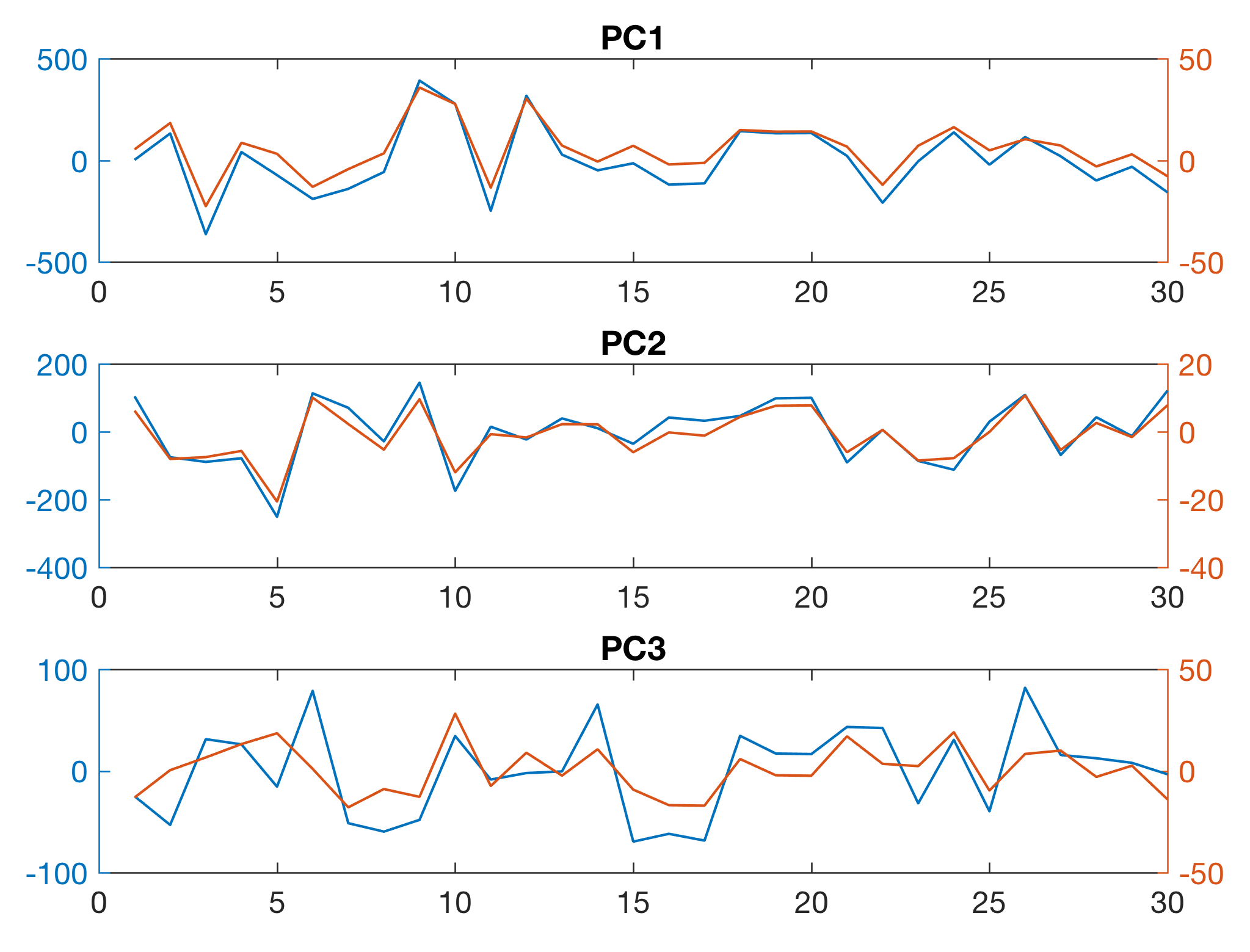
We can estimate the quality of the result by comparing the initial variations in s1, s2 and s3 with the (more or less) independent variables PC1, PC2 and PC3 stored in the three columns of newx.
subplot(3,1,1)
plotyy(1:30,newx(:,1),1:30,s1)
title('PC1')
subplot(3,1,2)
plotyy(1:30,-newx(:,2),1:30,s2)
title('PC2')
subplot(3,1,3)
plotyy(1:30,newx(:,3),1:30,s3)
title('PC3')
The sign and the amplitude cannot be determined quantitatively and therefore, in this case, we change the sign of the second PC and use plotyy to display the data on different axes in order to compare the results (in blue color). As we can see, we have successfully unmixed the varying contributions of the source rocks s1, s2 and s3 (in red color) to the mineral composition of the sedimentary sequence.
More details about the method and the interpretation of the loads, the scores and the variance explained is contained in the MRES book. The book also includes a section about the ICA as an alternative to the PCA for unmixing non-Gaussian data.
References
Hotelling H (1931) Analysis of a Complex of Statistical Variables with Principal Components. Journal of Educational Psychology 24(6):417-441
Pearson K (1901) On lines and planes of closest fit to a system of points in space. Philosophical Magazine and Journal of Science 6(2):559–572